An inference engine for RDF

Author: G.Naudts

Mail adress: naudts_vannoten@yahoo.com

RDF is a system meant for stating meta-information i.e. information that says something about other information e.g. a web page. RDF works with triples. A triple is composed of an subject, a property and an object. A complication is that subject and object can be either the designation of something (a URI like http://www.example/person) or a set of triples.

Fig.1 gives an example of triples.

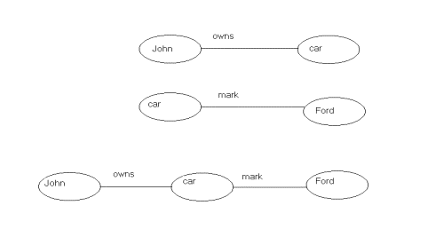
Fig.1 Some RDF triples.

Triples can be ‘stand-alone’ or they can form a graph. The first triple says that John owns a car and the second says that there is a car with mark Ford. The third drawing however is composed of two triples (and is thus a triple set) and it says that John owns a car with mark Ford. (By the way this is the graph representation of triples). As was said above subject and object can be a set of triples meaning that every node in the graph can be again a graph.

Suppose fig.1 represents the database. Now let’s make a query. Fig.2 gives the representation of some queries.

In the first query the question is: who owns a car? The answer is of course “John”. In the second query the question is: what marks of car are defined in the database?

The third query however asks: who owns a car and what is the mark of that car?

Here the query is a graph containing variables. This graph has to be matched with the graph in fig.1. Should the graph in the db be more extended it would have to be matched with a subgraph. So generally for executing a RDF query what has to be done is “subgraph matching”.

Following the data model for RDF the two queries are in fact equal because a sequence of statements is implicitly a conjunction. Fig.3 illustrates this.

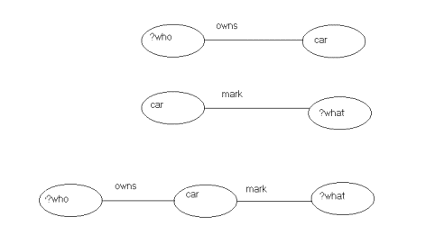
Fig.2. Some RDF queries.

Fig. 3.An erroneous sequence of statements.

Through the implicit conjunction the first sequence of triples constitutes a faulty database. John’s car cannot have two different marks.

Suppose there exists a rule: if X owns a car then that X must pay taxes. How to represent such a rule ? Fig.4 gives the graph representation of a rule.

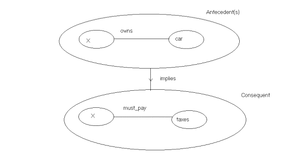
Fig.4. The graph representation of a rule. A representation in line with prolog rules.

The nodes of the rule form a triple set. Here there is one antecedent but there could be more. There is only one consequent. (Rules with more than one consequent can be reduced to rules with one consequent). Fig.5 gives a query that will match with the consequent of the rule.

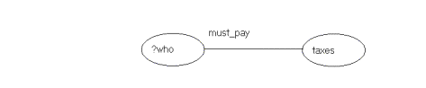
Fig. 5. A query that matches with a rule.

The desired answer is of course: John must pay taxes. The query of fig.5 is matched with the consequent of the rule in fig.4. Now an action has to be taken: the antecedents of the rule have to be added to the database with the variables replaced with the necessary values (substitution). Then the query has to be continued with the antecedent of the rule. The question now is: who owns a car? This is equal to a query described earlier. Important is that a rule subgraph is treated differently from non-rule subgraphs.

How to execute these queries using the theory of first-order resolution?

A triple can be modeled as a predicate: Triple(subject, property, object). A set of triples = a list of triples. A connected graph is decomposed into a set of triples. For the examples above this gives(lists are between []):

Fig.1:

Triple(John, owns, car).

Triple(car, mark, Ford).

This sequence is equivalent to:

[Triple(John, owns, car). Triple (car, mark, Ford).]

Fig.2:

Triple(?who, owns, car).

Triple(car, mark, ?what).

This sequence is equivalent to:

[Triple(?who, owns, car). Triple(car, mark, ?what).]

Fig.3:

Triple([Triple(X, owns, car)], implies, [Triple(X, must_pay, taxes)]).

Fig.4: Triple(?who, must_pay, taxes).

These predicates can be represented e.g. in prolog.

But the query [Triple(?who, owns, car). Triple(car, mark, ?what).] cannot be executed in Prolog because prolog will do no subgraph matching. The DB might contain the clause: [Triple(car, mark, Ford). Triple(John, wife, Mary). Triple(John, owns, car)]. This clause will not match with the query above. The order of triples in a list of triples has no relevance.

Another problem are rules: the rule of fig. 4 can become in prolog:

Triple(X, must_pay, taxes) :- Triple(X, owns, car)

But rules in rdf can be embedded:

Triple([Triple([Triple(level, =, “20”)],implies,[Triple(alarm, level, one)])], implies,[Triple(level, =, 10)]). Or more informally:

((level = 20) à (alarm level one)) à (level = 10)

The meaning: when the level has reached 10 a rule is generated that says that, when the level is 20 an alarm of level one must be given. This permits the dynamic generation of rules.

. What is this in prolog?

Reduced to conjunctive normal form it can be seen that this is not a horn clause.

It can be handled by Otter, a theorem prover, who permits first-order logic in conjunctive normal form. However subgraph matching is not possible in Otter without programming.

So I have developed a unification algorithm for RDF that can handle subgraph matching and embedded rules. It can be characterised by the term: “subgraph matching with rules”.

Fig. 6 gives an overview of the unification algorithm.

It works as follows: the sequence of RDF statements is divided into sets where each set constitutes a connected subgraph. This is called a tripleset. This division is done for the database and for the query. Then the algorithm tries to match each tripleset (= subgraph) of the query with each tripleset (=subgraph) of the database. Each triple of a tripleset of the query is matched with each triple of the tripleset of the database. All the triples of the query set must be unifiied with a triple from the database. If one triple is a rule unification will use the mechanism for rules.

Note: the modeling of a triple e.g. by owns(John, car) in prolog is not correct because the predicate can be a variable too.

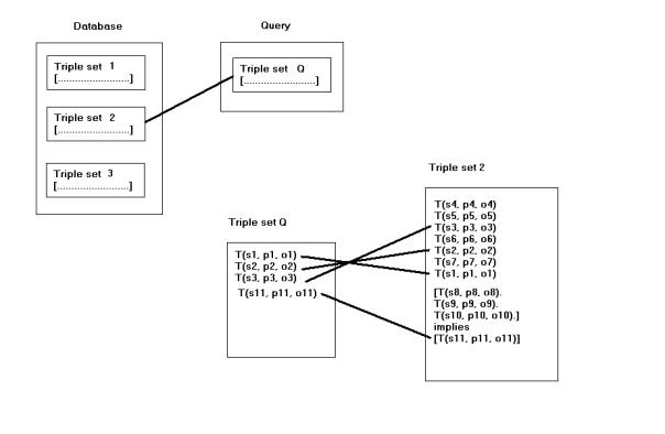
Fig. 6. The unification algorithm.

This algorithm is very well suited for working with graphs: a graph can be declared by triples and rules can do inferencing about properties of graphs. A complex description of the nodes is possible because each node can be a graph itself.

Some complications

1) Multiple matches in one triple set

Fig.7 gives a schematic view of multiple matches of a triple with a triple set. The triple T(Bart, son, ?w) unifies with two triples T(Bart, son, Jan) and T(Bart, son, Michèle). The triple T(?w, son, Paul) matches with T(Guido, son, Paul) and T(Jan, son, Paul). This gives 4 possible combinations of matching triples. Following the theory of resolutions all those combinations must be contradicted. However, the common variable ?w between the first and the second triple of triple set 1 is a restriction. The object of the first triple must be the same as the subject of the second triple with as a consequence that there is one solution: ?w = Jan. Suppose the second triple was: T(?w1, son, Paul). Then this restriction does not any more apply and there are 4 solutions:

[T(Bart, son, Jan), T(Guido, son, Paul)]

[T(Bart, son, Jan], T(Jan, son, Paul)]

[T(Bart, son, Michèle), T(Guido, son, Paul)]

[T(Bart, son, Michèle), T(Jan, son, Paul)]

This example shows that when unifying two triple sets the product of all the alternatives has to be taken while the substitutions have to be propagated from one triple to the next for the variables that are equal.

Two remarks:

1) This algorithm can be implemented by a resolution process with backtracking.

2) The triple sets can contain variables; the algorithm amounts to the search of all possible subgraphs of a connected graph, where the possible subgraphs are defined by the triples and the variables in the first triple set.

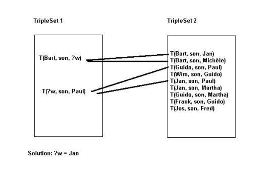
Fig.7. Multiple matches within one TripleSet.

2) Matching a triple set with a rule

The interpretation of a rule in the graph model of RDF and in resolution inferencing at the same time is:

When a triple that has to be contradicted matches with the consequent it is replaced by the tripleset (= subgraph) constituted by the antecedents. Now it is the subgraph consisting of the antecedents that has to be contradicted. Fig.8 shows the situation. T(Guido, parent, ?w1) matches with the consequent. This triple is replaced by the antecedents i.e. [T(?a, child, ?b)]. However all the triples in triple set 1 have to be unified. So the set of alternatives is triple set 1 with the triple T(Guido, parent, ?w1) replaced by T(?a, child, ?b) with the substitution: ?b = Guido.

Fig.8. Interpretation of a rule.

The semantic interpretation of a rule

The model theory of rdf describes entailment on a graph G. Simply said, a graph G entails a subgraph S.

Take the following rule R:

[T( ?c1, subClassOf, ?c2), T( ?c2, subClassOf, ?c3)] à T( ?c1, subClassOf , ?c3).

The rule is applied to all sets of triples in the graph G:

[T(c1, subClassOf, c2), T(c2, subClassOf, c3)]

yielding a triple T(c1, subClassOf, c3).

This last triple is then added to the graph. This process continues till no more triples can be added. A graph G’ is obtained called the closure of G with respect to the rule R.

If a query is posed: T(cx, subClassOf, cy) then the answer is positive if this triple is part of the closure G’; the answer is negative if it is not part of the closure.

When variables are used in the query:

T(?c1, subClassOf, ?c2)

then the solution consists of all triples (subgraphs) in the closure G’ with the predicate ‘subClassOf’.

The process is illustrated in fig. 9 with a similar example.

This gives following definitions:

A rule R is valid with respect to the graph G if its closure G’ with respect to the graph G is a valid rdf graph.

The graph G entails the graph T using the rule R if T is a subgraph of the closure G’ of the graph G with respect to the rule R.

When more than one rule is used the closure G’ will be obtained by the repeated application of the set of rules till no more triples are produced.

Any solution obtained by a resolution process is then a valid solution if it is a subgraph of the closure obtained.

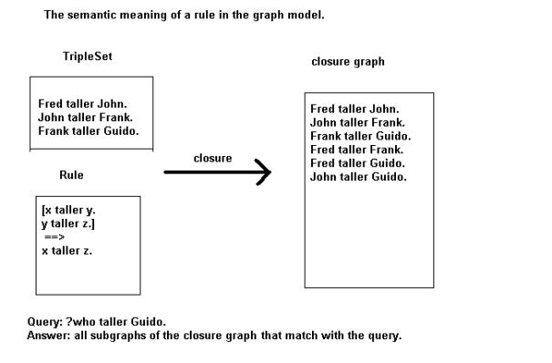
Fig. 9. The closure G’ of a graph G.

Unification

A triple is made of subject, property and object. Unifying two triples means unifying the two subjects, the two properties and the two objects. A variable unifies with a URI or a literal. Two URI’s unify if they are the same. The result of a unification is a substitution. A substitution is either a tuple (variable, URI or Literal) or nothing (an empty substitution). The result of the unification of two triples is a list of substitutions (maximally 3). Applying a substitution to a variable in a triple means replacing the variable with the URI or literal.

The resolution process

The resolution process starts with a query. A query is a tripleset. The query will be matched against the triplesets of the initial graph G and against the rules. The set unifies with a rule when one of the triples of the set unifies with the consequent of the rule. The set unifies with another set if all triples in the set unify with a triple of the other set. This can possibly be done in different ways. The result of the unification of two triple sets is a list of substitutionlists.

A triple set may unify with many other triple sets or rules.

The unification with a triple set from the graph G gives a substitution plus grounded triples. No new goals are returned as subgraph matching with the original graph has occurred. The unification with a rule has as a result one or more triplesets. Each tripleset is a new goal. Each of these new goals will be the continuation of a different search path. One of these paths will be further investigated and after a unification will split again into other paths or stop with a failure. The other paths will be pushed on a stack to be investigated later. It is easy to see that these search paths form a tree. In a depth first search the search goes on following one path till a leaf of the tree is met. Then backtracking is done one level in the tree and the search goes on till a new leaf is met.

In a breadth first search for all paths one unification is done, one path after another. All paths are followed at the same time till, one by one, they reach an endpoint.

Structure of the engine

The inference engine : this is where the resolution is executed. There are three parts to this engine:

a) solve : the generation of new goals by selection of a goal from the goallist by some selection procedure and unifying this goal against all blocks of the database thereby producing a set of alternative blocks. If the goallist is empty a solution has been found and a backtrack is done in search of other solutions.

b) choose: add one of the alternative blocks to the goallist; the other ones are pushed on the stack. Each set of alternative goals is pushed on the stack together with the current goallist and the current substitution. If solve did not generate any alternative goals there is a failure (unification did not succeed) and a backtrack must be done to get an alternative goal.

c) backtrack: an alternative goal is retrieved from the stack and added to the goallist. If the stack is empty the resolution process is finished. A failure occurs if for none of the alternatives a unification is possible; otherwise a set of solutions is given.

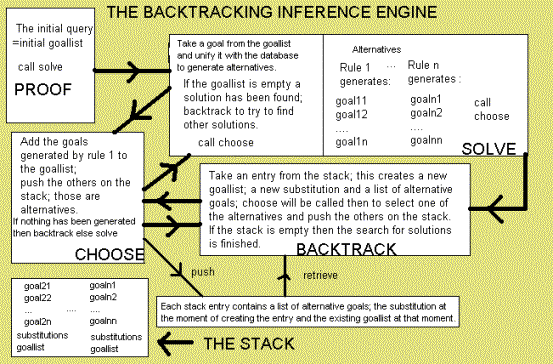
Fig.10. A schematic overview of the backtracking engine.

What is called above a substitution is a set of transformations of variable and atoms into variables and atoms. For each solution to a query there exists such a set of transformations that will transform the variables in the query into grounded atoms. Thus in fact the answer to the query is a list of substitutions = a list of lists of transformations.

The backtracking resolution mechanism in pseudo-language

Note: a block = a set of triples is what corresponds in prolog to a clause.

goalList = all blocks in the query.

do {

while (! goalList = empty) {

select a goal.

If this goal is a new goal unify this goal against the database producing a set of alternative goals ( = all the blocks which unify with the selected goal) and eliminate this goal from the goalList

else the engine is looping; backtrack to the proper choicepoint.

add one of this alternative set to the goalList and push the others on the stack

} // while

retrieve an alternative from the stack

} until (stack == empty)

The goal which is selected from the goalList is the head of the goalList. The alternative which is chosen from the list of alternatives is the first alternative in the list.

The mechanism which is followed is in fact SLD-resolution: Selection, Linear, Definite. There is a selection function for blocks; a quit simple one given the fact that the first in the list is selected (here is one of the point where optimisation is possible namely by using another selection function); linear means that the resolution rule is followed. In prolog the definition of a definite sentence is a sentence that has exactly one positive literal in each clause and the unification is done with this literal. In the N3-database rules have exactly one “positive block” which is the consequent and facts always are a positive block.

Following resolution strategies are respected by an SLD-engine:

· depth first: each alternative is investigated until a unification failure occurs or until a solution is found. The alternative to depth first is breadth first.

· set of support: at least one parent clause must be from the negation of the goal or one of the “descendents” of such a goal clause. This is a complete procedure that gives a goal directed character to the search.

· unit resolution: at least one parent clause must be a “unit clause” i.e. a clause containing a single literal. This is not generally complete, but complete for Horn clauses. Is this complete for N3?

· input resolution: at least one parent comes from the set of original clauses (from the axioms and the negation of the goals). This is not complete in general but complete for Horn clause KB's.Is this complete for N3 KB’s?.

· linear resolution: the general resolution rule is followed.

· ordered resolution: this is the way prolog operates; the clauses are treated from the first to the last and each single clause is unified from left to right.

The closure path.

A rule is applied to a graph G; the antecedents of the rule are matched with one or more subgraphs of G to yield a consequent that is added to the graph G. The consequent must be grounded for the graph to stay a valid rdf graph. This means that the consequent can not contain variables that are not in the antecedents.

Formally:

1) g1 (r1) à (s1, c1) where g1 is a subgraph of G, r1 is a rule; s1 is a substitution and c1 is the substituted consequent. This formula is called a rule application.

A full closure path is a sequence of rule applications where sometimes for clarity the term à (s1, c1) can be omitted.

Fig. 11, 12 and 13 give an example of closure paths.

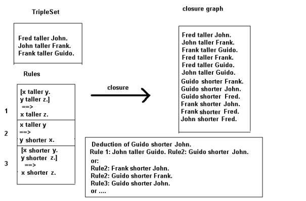
Fig.11. Example of closure paths. The first path consists of the application of rule 1 and rule2; the second of rule2, rule2 and rule3.

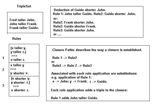
Fig.12. Description of closure paths.

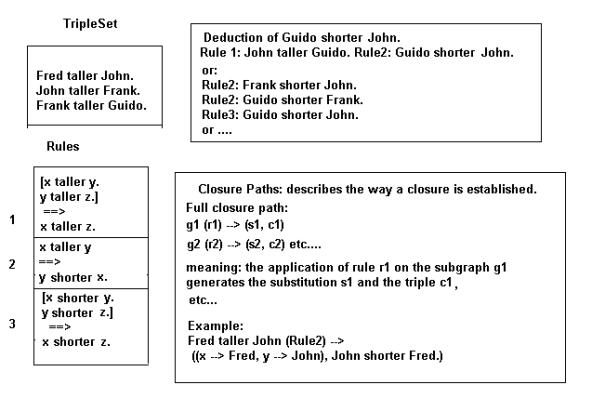
Fig.13. The notation for a closure path description.

The resolution path.

A rule is applied to a subgraph g1 (a goal) with result

- a substitution s and a tripleset g1’

- g1 is unified with a connected subgraph of G with result a substitution s1 and no subgraph in return.

Formally:

2) g1 (r1) à (s1, g1’) for a rule

3) g1 () à (s1, nil) for a subgraph match

The ‘()’ can be considered to be a ‘nil’-rule i.e. a rule without antecedents.

A full resolution path is a sequence of formulas 2 and 3. The parts with the à can be omitted for clarity.

Fig. 14 and fig.15 give some examples. The second example shows how even with a simple db and some rules the process is not so easy to follow. The resolution process cannot be executed on the data shown in fig.14: the variables must be renamed (or renumbered); if not, substitutions will be mixed up.

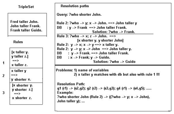
Fig.14. Examples of resolution paths. For understanding the second example best read the paragraph on variable renaming!!!

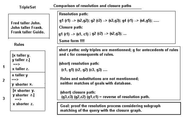
Fig.15. The notation for a resolution path.

Variable renaming

There are two reasons why variables have to be renamed when applying the resolution process (fig. 16):

1) Different names for the variables in different rules. Though it is permitted to define the rules using the same variables the inference process cannot work with this. Rule one rule might give a substitution xàFrank and later on in the resolution process rule two might give a substitution x à John. So by what has x to be replaced?

It is possible to program the resolution process without this renumbering but I think it’s a lot more complicated than renumbering the variables in each rule.

2) Take the rule:

[x1 taller y1. y1 taller z1.] à x1 taller z1.

At one moment ‘John taller Fred’ matches with ‘x1 taller z1’ giving substitutions:

x1 à John; z1 à Fred.

Later in the process ‘Fred taller Guido’ matches with ‘x1 taller z1’ giving substitutions:

x1 à Fred; z1 à Guido.

So now, by what is x1 replaced? Or z1?

This has as a consequence that the variables must receive a level numbering where each step in the resolution process is attributed a level number.

The substitutions above then become e.g.

1_x1 à John; 1_x1 à Fred

and

2_x1 à Fred, 2_z1 à Guido

This numbering is mostly done by prefixing with a number as done above. The variables can be renumbered in the database but it is more efficient to do it on a copy of the rule before the unification process.

In some cases this renumbering has to be undone e.g. when comparing goals.

The goals:

Fred taller 1_x1.

Fred taller 2_x1.

are really the same goals: they represent the same query: all people shorter than Fred.

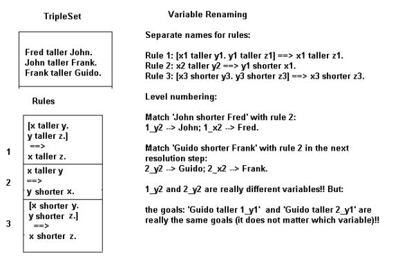
Fig. 16. Example of variable renumbering.

Comparison of resolution and closure paths

There is clearly a likeness between closure paths and resolution paths. As well for a closure path as for a resolution path there is a sequence of couples gx (rx) where () is considered to be a kind of 0 rule. In fact parts of the closure process are done in reverse in the resolution process.

Question: is it possible to find criteria such that steps in the resolution process can be judged to be valid based on (steps in ) the closure process?

If a rule is applied in the resolution process to a triple set and one of the triples is replaced by the antecedents then schematically:

c à as

where c represent the consequent and as the antecedents.

In the closure process there might be a step:

as à c where c is generated by the subgraph as.

[Or as à nil as the reverse of a direct match in the resolution process with the graph: nil à as. ]

If from a resolution path only that information is kept that corresponds to the steps c à as and this is called a short resolution path, in short resolution path, and from a closure path only the information is kept that corresponds to the steps as à c and this is called a short closure path, in short closure path, then the reverse of a closure path is a resolution path. (I will omit the ‘short’ in the notation from now on).

Example: closure path: (g1, c1) (g2,c2) (g3,c3). The gi are subgraphs (triple sets) who generate by a rule a triple ci that is added to the graph.

The reverse is: (c3, g3) (c2, g2) (c1, g1) and is a resolution path. A goal is matched with the ci to produce the alternatives gi.

The resolution path is that part of the inferencing process that is needed to inference triples or subgraphs that are not part of the original graph G and that thus are produced by the closure.

A closure path generates a solution when the query matches with a subgraph of the closure produced by the closure path.

Final Path Lemma(part): a final resolution path is always the reverse of a closure path.

A final resolution path is the resolution path when the goal list has been emptied and a solution has been found.

In a first instance only queries will be considered that are simple triples.

Take a sequence q (r1) g1 () Thus the query matches once with rule r1 to generate subgraph g1 who matches with graph G. This corresponds to the closure path: g1 (r1) q () where q in the closure G’ is generated by rule r1.

Example: Graph G :

[chimp subClassOf monkeys. monkeys subClassOf mammalia.]

And the subclassof rule:

[c1 subClassOf c2. c2 subClassOf c3.] à c1 subClassOf c3.

- The closure generates using the rule:

chimp subClassOf mammalia.

and adds this to the database.

- The query:

chimp subClassOf ?who.

will generate using the rule :

[chimp subClassOf c2. c2 subClassOf c3.]

and this matches with the database where c2 is substituted by monkeys and c3 is substituted by mammalia.

Proof:

Take the resolution path:

(c3, g3) (c2, g2) (c1, g1)

The last triple set (g1) unifies with the graph G. Would this not be the case it should either fail or unify with a rule. None of these is the case: it is the result of the last rule applied and there has been no failure.

The rules applied in sequence are r1, r2, and r3;

The reverse path is: (g1, c1) (g2, c2) (g3, c3).

g1 is grounded as was already established. The application of rule r1 to g1 will yield a grounded triple c1.

In the tuple (c2,g2) of the resolution path g2 is generated by application of the rule r2 on c2. The triples of g2 match either with G or one of the triples is c1 with the rule r1 applied to it. In both cases all the triples are grounded. The same reasoning can be applied to the tuple (c3, g3) where the triple c3 is part of the query.

Solution Lemma I: A solution corresponds to an empty closure path (when the query matches directly with the db) or to one or more minimal closure paths.

Note: a minimal closure path with respect to a solution consists of the minimum steps that are necessary for the closure to contain this solution.

Proof: there are two possibilities: the triples of a solution either belong to the graph G or are generated by the closure process. If all triples belong to G then the closure path is empty. If not there is a closure path that generates the triples that do not belong to G. QED.

It is clear that there can be more than one closure path that generates a solution. One must only consider applying rules in a different sequence. As the reverse of the closure path is a final resolution path it is clear that solutions can be duplicated during the resolution process.

Query Lemma: in a minimal closure path that generates a solution the last triple is a part of the query.

Proof: be (g1,c1) (g2,c2) (g3, c3) a closure path

Now c3 must unify with the query otherwise the step (g3,c3) should not be necessary in the closure.

Solution Lemma II: be C the set of all closure paths that generate solutions. Then there exist matching resolution paths that generate the same solutions.

Proof: be (g1,c1) (g2, c2) (g3, c3) a closure path that generates a solution.

Let (c3, g3) (c2, g2) (c1, g1) be the corresponding resolution path.

The applied rules are called r1, r2, r3.

r3 applied to c3 gives g3. Some of the triples of g3 can match with G, others will be deduced from further inferencing (for instance one of them might be c2).When c3 was generated in the closure it was deduced from g3. The triples of g3 can be part of G or they were derived with rules r1 and r2. If they were derived then the resolution process will use those rules to inference them in the other direction. If a triple is part of G in the resolution process it will be directly matched with a corresponding triple from the graph G.

The resolution path is a valid resolution path if after substitution the query is grounded or the resolution can be continued till the query is grounded.

The resolution path is invalid when it is not valid.

The resolution path is complete when after substitution all triples in it are grounded.

Final Path Lemma(part): A final resolution path always represents a solution.

Proof: Be (c1,g1) .. (cx,gx) .. (cn,gn) a final resolution path. gn is a subgraph of G (if not, the tuple (cn, gn) should be followed by another one). c1 is necessarily a triple of the query. The other triples of the query match with the graph G or or equal to ci, cj etc.. (consequents of a rule). The reverse is a closure path (final path lemma, above).However this closure path generates all triples of the query that did not match directly with the graph G. Thus it generates a solution. QED.

Anti-looping technique

The technique described here stems from an oral communication of Deroo [DEROO]. Given a full resolution path: q (r1) g1 (r2) g2 …. gn. Suppose the goal gn matches with the rule rn to generate the goal gn+1. When that goal is identical to one of the goals already present in the resolution path and generated also by the same rule rn then a loop may exist where the goals will keep coming back in the path.

This gives the resolution path e.g.

q (r1) g1 (r2) g2 … (r1) g1 (rn) gn (r1) g1 ….

This path is looping when the sequence g1 (r1) comes back for the second time and the environment is the same i.e. the current substitution is the same. (However replacing variables by variables with the same name but a different level number should not count for a different substitution).

The anti-looping technique consists in failing such a path from the moment a sequence (rx) gx comes back for the second time.

No solutions are excluded by this technique as shown by the solution lemma II. Indeed the reverse of a looping path is not a closure path. But there exists closure paths whose reverse is a resolution path containing a solution. So all solutions can still be found by finding those paths.

However if a goal returns but generated by another rule this rule must not fail e.g.

q (r1) g1 (r2) g2 …gn (rx) g1 …

Here the reverse path:

g1 (rx) gn… g2 (r2) g1 (r1) q

is a valid closure path because, of course, a different rule may be applied to an existing triple to add a new triple to the graph. However this new triple should not really be added to the list of goals because its validity will have to be proofed anyway.

In the implementation a list of goals should be kept. This list must keep track of the current resolution level; when backtracking goals with higher level than the current must be token away.

Failure

A failure (i.e. when a goal does not unify with facts or with a rule) does never exclude solutions. Indeed the reverse of a failure resolution path can never be a closure path. Indeed the last triple set of the failure path is not included in the closure. If it were its triples should either match with a fact or with the consequent of a rule.

Completeness

Each solution found in the resolution process corresponds to a resolution path. Be S the set of all those paths. Be S1 the set of the reverse paths which are valid closure paths. The set S will be complete when the set S1 contains all possible closure paths generating the solution. This is the case in a resolution process that uses depth first search as all possible combinations of the goal with the facts and the rules of the database are tried.

In the formal part definitions are given and the lemmas above and others are proofed.

Fig. 16 gives an overview of the lemmas and the most important points proofed by them.

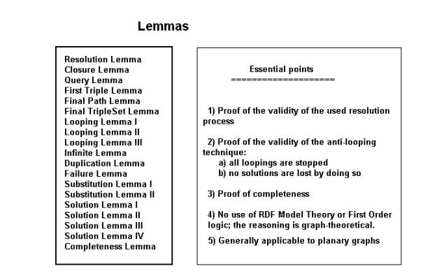
Fig.16. Overview of the lemmas.

A formal theory of graph resolution

Definitions:

A triple consists of two labeled nodes and a labeled arc.

A rule consists of antecedents and a consequent. The antecedents are a triple set; the consequent is a triple.

Applying a rule r to a graph G is the process of unifying the antecedents with all possible triples of the graph G while propagating the substitutions. For each successful unification the consequent of the rule is added to the graph with its variables substituted.

A rule r is valid with respect to the graph G if its closure G’ with respect to the graph G is a valid graph.

The graph G entails the graph T using the rule R if T is a subgraph of the closure G’ of the graph G with respect to the rule R.

The closure G’ of a graph G with respect to a ruleset R is the result of the application of the rules of the ruleset R to the graph G giving intermediate graphs Gi till no more new triples can be generated. A graph may not contain duplicate triples.

The closure G’ of a graph G with respect to a closure path is the resulting graph G’ consisting of G with all triples added generated by the closure path.

The solution to a query with respect to a graph G and a ruleset R is the set of all possible subgraphs of the closure that are the result of all possible unifications of the query with the closure G’ of G.

A rule is applied to a subgraph g1 (a goal) with result a substitution s and a tripleset g1’or g1 is unified with a connected subgraph of G with result a substitution s1 and o subgraph in return.

Formally:

2) g1 (r1) à (s1, g1’) for a rule

3) g1 () à (s1, nil) for a subgraph match

The ‘()’ can be considered to be a ‘nil’-rule i.e. a rule without antecedents.

A full resolution path is a sequence of formulas 2 and 3. The parts with the à can be omitted for clarity.

1) g1 (r1) à (s1, c1) where g1 is a subgraph of G, r1 is a rule; s1 is a substitution and c1 is the substituted consequent. This formula is called a rule application.

A short resolution path (abbreviated resolution path) is a sequence of tuples, each tuple consisting of a triple (consequent) and a triple set (antecedents) of a certain rule.

e.g. (q, g1) (c2, g2) (c3, g3).

A full closure path is a sequence of rule applications where sometimes for clarity the term à (s1, c1) can be omitted.

A short closure path (abbreviated closure path) is a sequence of triples each tuple consisting of a triple set (antecedents) and a triple (consequent) of a certain rule e.g. (g1, c1) (g2, c2) (g3, c3).

A minimal closure path with respect to a solution consists of the minimum steps that are necessary for the closure to contain this solution.

The graph generated by a closure path consists of the graph G with all triples added generated by the rules used for generating the closure path.

A closure path generates a solution when the query matches with a subgraph of the graph generated by the closure path.

The reverse of a closure path (g1, c1) … (gx, cx) … (gn, cn) is:

(cn, gn) … (cx, gx) … (c1, g1) and is a resolution path. .

A valid resolution path is a path where the triples of the query become grounded in the path after substitution or match with the graph G or the resolution process can be further applied to the path so that finally a path is obtained that contains a solution. All resolution paths that are not valid are invalid resolution paths. The resolution path is incomplete if after substitution the triple sets of the path still contain variables. The resolution path is complete when, after substitution, all triple sets in the path are grounded.

A final resolution path is the path that rests after the goallist in the (depth first search) resolution process has been emptied. The path then consists of all the rule applications applied during the resolution process.

A looping resolution path is a path with a recurring sequence (ri) gi e.g. q (r1) g1 … (rx) gx …. (rx) gx …

The resolution process is the building of resolution paths. A depth first search resolution process based on backtracking is explained elsewhere in the text.

Resolution Lemma. There are three possible resolution paths:

1) a looping path

2) a path that stops and generates a solution

3) a path that stops and is a failure

Proof. Obvious.

Closure lemma. The reverse of a closure path is a valid, complete and final resolution path for a certain set of queries.

Proof. Take a closure path: (g1,c1) … (gx,cx) … (gn,cn). This closure path adds the triples c1, …,cn to the graph. All queries that match with these triples and/or triples from the graph G will be proofed by the reverse path:

(cn, gn) … (cx, gx) … (c1,g1). The reverse path is complete because all closure paths are complete. It is final because the triple set g1 is a subgraph of the graph G (it is the starting point of a closure path). Take now a query as defined above: the triples of the query that are in G do of course match directly with the graph. The other ones are consequents in the closure path and thus also in the resolution path. So they will finally match or with other consequents or with triples from G.QED.

Query Lemma. In a minimal closure path that generates a solution the last triple is a part of the query.

Proof. Be (g1,c1) (g2,c2) (g3, c3) a closure path.

Now c3 must unify with the query otherwise the step (g3,c3) should not be necessary in the closure.

First Triple Lemma. The first triple in a resolution path must be a triple of the query triple set.

Proof. Obvious, because the process starts with the query.

Final Path Lemma. The reverse of a final path is a closure path. All final paths are complete and valid.

Proof. Be (c1,g1) … (cx,gx) …(cn-1,gn-1) (cn, gn) a final path.

c1 must be a triple of the query. gn on the other hand must belong to the graph G because, otherwise, it is or a failure path or a looping path.

Be (gn, cn) (gn-1,cn-1) … (gx, cx) … (g1, c1) the reverse path. The rule rn will generate from gn the triple cn that will be grounded. In the resolution process the triples from gn-1 either match with the graph G or one of them is cn. In both cases they will be grounded. Going on like this it is established that all triples are grounded in the resolution path. However all triples of the query either match with the graph G or are antecedent of a rule. In the first case they are in the closure G’, in the second case they are derived in the closure path and also in G’. Therefore the final path is also valid. It is complete by the closure lemma.

Final Tripleset Lemma. The last triple set in a final path is a subgraph of the original graph G.

Proof. This follows from the Final Path Lemma and the fact that the last goal in the goal list must match with a set from the graph G.

Looping Lemma I. If a looping resolution path contains a solution, there exists another non looping resolution path that contains the same solution.

Proof.

All solutions correspond to closure paths in the closure graph G’ (by definition). The reverse of such a closure path is always a valid resolution path and is non-looping. QED.

Looping Lemma II. A looping resolution path is never complete.

Proof. Be (c1, g1) …(cx,gx) …(cx, gx) … a looping path. The process starts with the query and everything that follows is generated by the triples of the query. The triples of the query can only become grounded when:

1) they match with a triple from the graph G.

2) after a certain path (c1,g1) ..(cn,gn) all gn become grounded.

However if this is true for all triples of the query, then the goallist must be empty and a solution found; thus there cannot be a loop. QED.

Looping Lemma III. Whenever the resolution process is looping, this is caused by a looping path if the closure of the graph G is not infinite.

Proof. Looping means in the first place that there is never a failure i.e. a triple or tripleset that fails to match because then the path is a failure path and backtracking occurs. It means also triples continue to match in an infinite series.

There are two sublemmas here:

Sublemma 1. In a looping process at least one goal should return in the goallist.

Proof.Can the number of goals be infinite? There is a finite number of triples in G, a finite number of triples that can be generated and a finite number of variables. This is the case because the closure is not infinite. So the answer is no. Thus if the process loops (ad infinitum) there is a goal that must return at a certain moment.

Sublemma 2. In a looping process a sequence (rule x) goal x must return. Indeed the numbers of rules is not infinite; neither is the number of goals; if the same goal returns infinitly, sooner or later it must return as a deduction of the same rule x.

QED.

Infnite Looping Path Lemma. If the closure graph G’ is not infinite and the resolution process generates an infinite number of looping paths then this generation will be stopped by the anti-looping technique and the resolution process will terminate in a finite time.

Proof. The finiteness of the closure graph implies that the number of labels and arcs is finite too.

Suppose that a certain goal generates an infinite number of looping paths.

This implies that the breadth of the resolution tree has to grow infinitely. It cannot grow infinitely in one step because each goal only generates an finite number of children (the DB is not infinite). This implies that also the depth of the resolution tree has to grow infinitely. This implies that the level of the resolution process grows infinitely and also then the number of entries in the oldgoals list.

Each growth of the depth produces new entries in the oldgoals list. (In this list each goal-rule combination is new because when it is not, a backtrack is done by the anti-looping mechanism). In fact with each increase in the resolution level an entry is added to the oldgoals list.

Then at some point the list of oldgoals will contain all possible rule-goals combinations and the further expansion is stopped.

Formulated otherwise, for an infinite number of looping paths to be materialized in the resolution process the oldgoals list should grow infinitely but this is not possible.QED.

Infinite Lemma. For a closure to generate an infinite closure graph G’ it is necessary that at least one rule adds new labels to the vocabulary of the graph.

Proof. Example: {:a log:math :n } à {:a log:math :n+1). The consequent generated by this rule is each time different. So the closure graph will be infinite. Suppose the initial graph is: :a log:math :0. So the rule will generate the sequence of natural numbers.

If no rule generates new labels then the number of labels and thus of arcs and nodes in the graph is finite and so are the possible ways of combining them.

Duplication Lemma. A solution to a query can be generated by two different valid resolution paths. It is not necessary that there is a cycle in the graph G’.

Proof. Be (c1,g1) (c2,g2) (c3,g3) and (c1,g1) (c3,g3) (c2,g2) two resolution paths.Let the query q be equal to c1. Let g1 consist of c2 and c3 and let g2 and g3 be subgraphs of G. Then both paths are final paths and thus valid (Final Path Lemma).

Failure Lemma. If the current goal of a resolution path (the last triple set of the path) can not be unified with a rule or facts in the database, it can have a solution, but this solution can also be found in a final path.

Proof. This is the same as for the looping lemma with the addition that the reverse of a failure path cannot be a closure path as the last triple set is not in the graph G (otherwise there would be no failure).

Substitution Lemma I. When a variable matches with a URI the first item in the substitution tuple needs to be the variable.

Proof. 1) The variable originates from the query.

a) The triple in question matches with a triple from the graph G. Obvious, because a subgraph matching is being done.

b) The variable matches with a ground atom from a rule.

Suppose this happens in the resolution path when using rule rx:

(c1, g1) … (cx, gx)

The goal is to find a closure path:

(gn, cn) … (gx,cx) … (g1,c1) where all atoms are grounded.

When rule rx is used in the closure the ground atom is part of the closure graph, thus in the resolution process , in order to find a subgraph of a closure graph, the variable has to be substituted by the ground atom.

3) a ground atom from the query matches with a variable from a rule. Again, the search is for a closure path that leads to a closure graph that contains the query as a subgraph. Suppose a series of substitutions:

(v1, a1) (v2,a1) where a1 originates from the query corresponding to a resolution path: (c1,g1) (c2,g2) (c3,g3). Wherever v1 occurs it will be replaced by a1. If it matches with another variable this variable will be replaced by a1 too. Finally it will match with a ground term from G’. This corresponds to a closure path where in a sequence of variables (v1, v2) from rules each variable becomes replace by a1, an atom of the initial graph.

4) a ground atom from a rule matches with a variables from a rule or the inverse. These cases are exactly the same as the cases where the ground atom or the variable originates from the query.

Substitution Lemma II. When two variables match, the variable from the query or goal needs to be ordered first in the tuple.

Proof. In a chain of variable substitution the first variable substitution will start with a variable from the query or a goal. The case for a goal is similar to the case for a query. Be a series of substitutions:

(v1,v2) (v2,vx) … (vx,a) where a is a grounded atom.

By applying this substitution to the resolution path all the variables will become equal to a. This corresponds to what happens in the closure path where the ground atom a will replace all the variables in the rules.

Solution Lemma I: A solution corresponds to an empty closure path (when the query matches directly with the db) or to one or more minimal closure paths.

Proof: there are two possibilities: the triples of a solution either belong to the graph G or are generated by the closure process. If all triples belong to G then the closure path is empty. If not there is a closure path that generates the triples that do not belong to G. QED.

Solution Lemma II: be C the set of all closure paths that generate solutions. Then there exist matching resolution paths that generate the same solutions.

Proof: be (g1,c1) (g2, c2) (g3, c3) a closure path that generates a solution.

Let (c3, g3) (c2, g2) (c1, g1) be the corresponding resolution path.

The applied rules are called r1, r2, r3.

Solution Lemma III. The set of all valid solutions to a query q with respect to a graph G and a ruleset R is generated by the set of all valid resolution paths, however with elimination of duplicates.

Proof.

A valid resolution path generates a solution. Because of the completeness lemma the set of all valid resolution paths must generate all solutions. But the duplication lemma states that there might be duplicates.

Solution Lemma IV. A complete resolution path generates a solution and a solution is only generated by a complete, valid and final resolution path.

Proof. à : be (c1,g1) … (cx,gx) … (cn,gn) a complete resolution path. If there are still triples from the query that did not become grounded by 1) matching with a triple from G or 2) following a chain (c1,g1) …(cn,gn) where all gn match with G, the path cannot be complete. Thus all triples of the query are matched and grounded after substitution, so a solution has been found.

ß : be (c1,g1) … (cx,gx) … (cn,gn) a resolution path that generates a solution. This means all triples of the query have 1) matched with a triple from G or 2) followed a chain (c1,g1) …(cn,gn) where gn matches with a subgraph from G. But then the path is a final path and is thus complete (Final Path Lemma). QED.

Completeness Lemma. The depth first search resolution process with exclusion of invalid resolution paths generates all possible solutions to a query q with respect to a graph G and a ruleset R.

Proof.

Each solution found in the resolution process corresponds to a closure path. Be S the set of all those paths. Be S1 the set of the reverse paths which are resolution paths (Valid Path Lemma). The set of paths generated by the depth first search resolution process will generate all possible combinations of the goal with the facts and the rules of the database thereby generating all possible final paths.

It is understood that looping paths are stopped.

An extension of the theory to variable arities

Definitions

A multiple of arity n is a predicate p also called arc and (n-1) nodes also called points. The points are connected by an (multi-headed) arc. The points and arcs are labeled and no two labels are the same.

A graph is a set of multiples.

Arcs and nodes are either variables or labels. (In internet terms labels could be URI’s or literals).

Two multiples unify when they have the same arity and their arcs and nodes unify.

A variable unifies with a variable or a label.

Two labels unify if they are the same.

A rule consists of antecedents and a consequent. Antecedents are multiples and a consequent is a multiple.

The application of a rule to a graph G consists in unifying the antecedents with multiples from the graph and, if successful, adding the consequent to the graph.

The lemmas of the theory explained above can be used if it is possible to reduce all multiples to triples and then proof that the solutions stay the same.

Reduction of multiples to triples:

Unary multiple: In a graph G a becomes (x1, x2, a) where x1 and x2 are unique labels that are recognizable as temporary labels. In a query a becomes (y1, y2, a) where y1 and y2 are variables.

If ?a matches with a then (y1, y2, a) matches with (x1, x2, a).

Binary multiple: (p,a) becomes (x1,p,a)? The query (?p,?a) corresponds with (y1, ?p, ?a).

Ternary multiple: this is a triple.

Quaternary multiple: (p, a, b, c) becomes:

{(x, p, a), (x, p, b), (x,p,c)} where x is a unique temporary label.

The query (?p,?a,?b,?c) becomes:

{(y,?p,?a),(y,?p,?b),(x,?p,?c)}.

It is quit obvious that this transformation does not change the solutions.

An extension of the theory to typed nodes and arcs

A sentence is a sequence of syntactic entities. A syntactic entity has a type and a label. Example: verb/walk.

Examples of syntactic entities: verb, noun, article, etc… A syntactic entity can also be a variable. It is then preceded by an interrogation mark.

A language is a set of sentences.

Two sentences unify if their entities unify.

A rule consists of antecedents that are sentences and a consequent that is a sentence.

An example: {(noun/?noun, verb/walks)} à {(article/?article,noun/ ?noun, verb/walks)}

In fact what is done here is to create multiples where each label is tagged with a type. Unification can only happen when the types of a node or arc are equal besides the label being equal.

Of course sentences are multiples and can be transformed to triples.

Thus all the lemmas from above apply to these structures if solutions can be defined to be subgraphs of a closure graph. .

This can be used to make transformations e.g.

(?ty/label,object/?ty1) à (par/’(‘, object/?ty1).

Parsing can be done:

(?/charIn ?/= ?/‘(‘) à (?/charOut ?/= par/’(‘)

[DEROO] http://www.agfa.com/w3c/jdroo

* the site of the Euler program

[JONES] http://www.haskell.org/hugs/demos/prolog The prolog demo in the Hugs distribution.

[RDFM]RDF Model Theory .Editor: Patrick Hayes

<http://www.w3.org/TR/rdf-mt/>

[TBL] Tim-berners Lee, Weaving the web,

[TBL01] Berners-Lee e.a.The semantic web, Scientific American May 2001

[WOS] Wos e.a. Automated reasoning,Prentice Hall, 1984