An inference engine for RDF
Master thesis
G.Naudts
831708907
22
augustus 2003
Open University Netherlands
Agfa Gevaert
This document is the Master Thesis made as a part of
my Master Degree in Computer Science Education (Software Systems) at the Open
University of the Netherlands. The work has been done in collaboration with the
research department of the company Agfa in Mortsel Belgium.
Student
data
Name Guido Naudts
Student number 831708907
Address Secretarisdreef 5
2288 Bouwel
Telephone work 0030-2-542.76.01
Home 0030-14-51.32.43
E-mail Naudts_Vannoten@yahoo.com
Coaching
and graduation committee
Chairman: dr J.T. Jeuring, professor at the Open
University
Secretary : ir. F.J. Wester, senior lecturer at the Open
University
Coach: ir. J. De Roo, researcher at Agfa
Gevaert.
Acknowledgements
I want to thank Ir.J.De Roo for giving me the opportunity for making a thesis about a tremendous subject and his guidance in the matter.
Pr.J.Jeuring and Ir. F.Wester are thanked for their efforts to help me produce a readable and valuable text.
I thank M.P.Jones for his Prolog demo in the Hugs distribution that has very much helped me.
I thank all the people from the OU for their efforts during the years without which this work would not have been possible.
I thank my wife and children for supporting a father seated behind his computer during many years.
Coaching and graduation
committee
1.2.3.Conclusions of the case study
1.6. Relation with the current research
Chapter
2. The building blocks
2.4.Resource Description Framework RDF
2.7.2. The model theory of RDF
2.8. A global view of the Semantic Web
2.8.2. The layers of the Semantic Web
Chapter
3. RDF, RDFEngine and inferencing.
3.2.Recapitulation and definitions
3.4.Languages needed for inferencing
3.5.The model interpretation of a rule
3.14.Comparison of resolution and closure
paths
3.17.A formal theory of graph resolution
3.18.An extension of the theory to variable
arities
3.19.An
extension of the theory to typed nodes and arcs
Chapter
4. Existing software systems
Chapter 5. RDF, inferencing
and logic.
5.2.3. A problem with reification
5.3.Unification
and the RDF graph model
5.4.Completeness and soundness of the engine
5.7. Comparison with Prolog and Otter
5.7.1. Comparison of Prolog with RDFProlog
5.8.Differences
between RDF and FOL
5.11. RDF and constructive logic
5.12.
The Semantic Web and logic
5.15.The
World Wide Web and neural networks
6.3. An optimization technique
7.3. OWL Lite and inconsistencies
7.5. Reactions to inconsistencies and trust
7.5.1.Reactions to inconsistency
7.5.2.Reactions to a lack of trust
8.4. Searching paths in a graph
8.6. Simulation of logic gates.
8.8. A simulation of a flight reservation
9.2.Characteristics
of an inference engine
9.3. An evaluation of the RDFEngine
9.4. Forward versus backwards reasoning
Appendix
1: Excuting the engine
Appendix 2. Example
of a closure path.
Simulation
of a flight reservation
Appendix
4. Theorem provers an overview
2.2 Reasoning using resolution techniques: see
the chapter on resolution.
2.5. The matrix connection method
Higher order interactive provers
Overview of different logic systems
3. First order predicate logic
5.
Modal logic (temporal logic)
6. Intuistionistic or constructive logic
Appendix
5. The source code of RDFEngine
Appendix
6. The handling of variables
Summary
The Semantic Web is
an initiative of the World Wide Web
Consortium (W3C). The goal of this project is to define a series of
standards. These standards will create a framework for the automation of
activities on the World Wide Web
(WWW) that still need manual intervention by human beings at this moment.
A certain number of basic standards have been
developed already. Among them XML is without doubt the most known. Less known
is the Resource Description Framework
(RDF). This is a standard for the creation of meta information. This is the
information that has to be given to computers to permit them to handle tasks
previously done by human beings.
Information alone however is not sufficient. In order
to take a decision it is often necessary to follow a certain reasoning.
Reasoning is connected with logics. The consequence is that computers have to
be fed with programs and rules that can take decisions, following a certain
logic, based on available information.
These programs and reasonings are executed by inference engines. The definition of
inference engines for the Semantic Web is at the moment an active field of
experimental research.
These engines have
to use information that is expressed following the standard RDF. The
consequences of this requirement for the definition of the engine are explored
in this thesis.
An inference engine
uses information and, given a query,
reasons with this information with a solution
as a result. It is important to be able to show that the solutions, obtained in
this manner, have certain characteristics. These are, between others, the
characteristics completeness and validity. This proof is delivered in
this thesis in two ways:
1)
by means of a
reasoning based on the graph theoretical properties of RDF
2)
by means of a
model based on First Order Logics.
On the other hand these engines must take into account
the specificity of the World Wide Web. One of the properties of the web is the
fact that sets are not closed. This implies that not all elements of a set are
known. Reasoning then has to happen in an open
world. This fact has far reaching logical
implications.
During the twentieth century there has been an
impetous development of logic systems. More than 2000 kinds of logic were
developed. Notably First Order Logic (FOL)
has been under heavy attack, beside others, by the dutch Brouwer with the constructive or intuistionistic logic. Research is also done into kinds of logic
that are suitable for usage by machines.
In this thesis I argue that an inference engine
for the World Wide Web should follow a kind of constructive logic and that RDF,
with a logical implication added,
satisfies this requirement. It is shown that a constructive approach is
important for the verifiability of the results of inferencing.
The structure of the World Wide Web has a
number of consequences for the properties that an inference engine should
satisfy. A list of these properties is established and
discussed.
A query on the World Wide Web can extend over more
than one server. This means that a process of distributed inferencing must be
defined. This concept is introduced in an experimental inference engine,
RDFEngine.
An important characteristic for an engine that has to
be active in the World Wide Web is efficiency.
Therefore it is important to do research about the methods that can be used to
make an efficient engine. The structure has to be such that it is possible to
work with huge volumes of data. Eventually these data are kept in relational
databases.
On the World Wide Web there is information available
in a lot of places and in a lot of different forms. Joining parts of this
information and reasoning about the result can easily lead to the existence of contradictions and inconsistencies. These are inherent to the used logic or are
dependable on the application. A special place is taken by inconsistencies that
are inherent to the used ontology. For the Semantic Web the ontology is
determined by the standards rdfs and OWL.
An ontology introduces a classification of data and apllies restrictions to those data. An inference engine for the Semantic Web needs to have such characteristics that it is compatible with rdfs and OWL.
An executable specification of an inference engine in Haskell was constructed. This permitted to test different aspects of inferencing and the logic connected to it. This engine has the name RDFEngine. A large number of existing testcases was executed with the engine. A certain number of testcases was constructed, some of them for inspecting the logic characteristics of RDF.
Samenvatting
Het Semantisch
Web is een initiatief van het World Wide
Web Consortium (W3C). Dit project beoogt het uitbouwen van een reeks van
standaarden. Deze standaarden zullen een framework scheppen voor de
automatisering van activiteiten op het World
Wide Web (WWW) die thans nog manuele tussenkomst vereisen.
Een bepaald aantal basisstandaarden zijn reeds ontwikkeld waaronder XML
ongetwijfeld de meest gekende is. Iets minder bekend is het Resource Description Framework (RDF).
Dit is een standaard voor het creëeren van meta-informatie. Dit is de
informatie die aan de machines moet verschaft worden om hen toe te laten de
taken van de mens over te nemen.
Informatie alleen is echter niet voldoende. Om een beslissing te kunnen
nemen moet dikwijls een bepaalde redenering gevolgd worden. Redeneren heeft te
maken met logica. Het gevolg is dat computers gevoed moeten worden met
programmas en regels die, volgens een bepaalde logica, besluiten kunnen nemen
aan de hand van beschikbare informatie.
Deze programmas en redeneringen worden uitgevoerd door zogenaamde inference engines. Dit is op het huidig
ogenblik een actief terrein van experimenteel onderzoek.
De engines
moeten gebruik maken van de informatie die volgens de standaard RDF wordt
weergegeven. De gevolgen hiervan voor de structuur van de engine worden in deze
thesis nader onderzocht.
Een inference
engine gebruikt informatie en, aan de hand van een vraagstelling, worden redeneringen doorgevoerd op deze informatie
met een oplossing als resultaat. Het
is belangrijk te kunnen aantonen dat de oplossingen die aldus bekomen worden
bepaalde eigenschappen bezitten. Dit zijn onder meer de eigenschappen volledigheid en juistheid. Dit bewijs wordt op twee manieren geleverd: enerzijds
bij middel van een redenering gebaseerd op de graaf theoretische eigenschappen
van RDF; anders bij middel van een op First Order Logica gebaseerd model.
Anderzijds dienen zij rekening te houden met de specificiteit van het
World Wide Web. Een van de eigenschappen van het web is het open zijn van verzamelingen.
Dit houdt in dat van een verzameling niet alle elementen gekend zijn. Het
redeneren dient dan te gebeuren in een open
wereld. Dit heeft verstrekkende logische implicaties.
In de loop van de twintigste eeuw heeft de logica een stormachtige
ontwikkeling gekend. Meer dan 2000 soorten logica werden ontwikkeld. Aanvallen
werden doorgevoerd op het bolwerk van de First
Order Logica (FOL), onder meer door de nederlander Brouwer met de constructieve of intuistionistische logica. Gezocht wordt ook naar soorten logica
die geschikt zijn voor het gebruik door machines.
In deze thesis wordt betoogd dat een inference engine voor het WWW een
constructieve logica dient te volgen enerzijds, en anderzijds, dat RDF
aangevuld met een logische implicatie
aan dit soort logica voldoet. Het wordt aangetoond that een constructieve
benadering belangrijk is voor de verifieerbaarheid van de resultaten van de
inferencing.
De structuur van het World Wide Web heeft een aantal gevolgen voor de
eigenschappen waaraan een inference engine dient te voldoen. Een lijst van deze
eigenschappen wordt opgesteld en besproken.
Een query op het World Wide Web kan zich uitstrekken over meerdere
servers. Dit houdt in dat een proces van gedistribueerde inferencing moet
gedefinieerd worden. Dit concept wordt geïntroduceerd in een experimentele
inference engine, RDFEngine.
Een belangrijke eigenschap voor een engine die actief dient te zijn in
het World Wide Web is efficientie.
Het is daarom belangrijk te onderzoeken op welke wijze een efficiente engine
kan gemaakt worden. De structuur dient zodanig te zijn dat het mogelijk is om
met grote volumes aan data te werken, die eventueel in relationele databases
opgeslagen zijn.
Op het World Wide Web is informatie op vele plaatsen en in allerlei
vormen aanwezig. Het samen voegen van deze informatie en het houden van
redeneringen die erop betrekking hebben kan gemakkelijk leiden tot het ontstaan
van contradicties en inconsistenties. Deze zijn inherent aan
de gebruikte logica of zijn afhankelijk van de applicatie. Een speciale plaats
nemen de inconsistenties in die inherent zijn aan de gebruikt ontologie. Voor
het Semantisch Web wordt de ontologie bepaald door de standaarden rdfs en OWL. Een ontologie voert een classifiering in van gegevens en legt
ook beperkingen aan deze gegevens op. Een inference engine voor het Semantisch
Web dient zulkdanige eigenschappen te bezitten dat hij compatibel is met rdfs
en OWL.
Een uitvoerbare specificatie van een inference
engine in Haskell werd gemaakt. Dit liet toe om allerlei aspecten van
inferencing en de ermee verbonden logica te testen. De engine werd RDFEngine
gedoopt. Een groot aantal bestaande testcases werd onderzocht. Een aantal
testcases werd bijgemaakt, sommige speciaal met het oogmerk om de logische
eigenschappen van RDF te onderzoeken.
Chapter 1. Introduction
1.1. Overview
In chapter 1 a case study is given and then the
goals of the research, that is the subject of the thesis, are exposed with the
case study as illustration. The methods used are explained and an overview is
given of the fundamental knowledge upon which the research is based. The
relation with current research is indicated. Then the structure of the thesis
is outlined.
1.2. Case study
1.2.1. Introduction
A case study can serve as a guidance to what we want
to achieve with the Semantic Web. Whenever standards are approved they should
be such that important case studies remain possible to implement. Discussing all possible application fields here
would be out of scope. However one case study will help to clarify the goals of
the research.
1.2.2. The case study
A travel agent in Antwerp has a client who wants to go
to St.Tropez in France. There are rather a lot of possibilities for composing
such a voyage. The client can take the train to France, or he can take a bus or
train to Brussels and then the airplane to Nice in France, or the train to
Paris then the airplane or another train to Nice. The travel agent explains the
client that there are a lot of possibilities. During his explanation he gets an
impression of what the client really wants. Fig.1.1. gives a schematic view of
the case study.
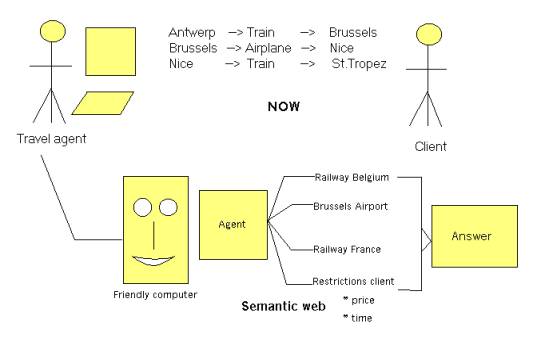
Fig.1.1. A Semantic
Web case study
He agrees with the client about the itinerary: by
train from Antwerp to Brussels, by airplane from Brussels to Nice and by train
from Nice to St. Tropez. This still leaves room for some alternatives. The
client will come back to make a final decision once the travel agent has said
him by mail that he has worked out some alternative solutions like price for
first class vs second class etc...
Remark that the decision for the itinerary that has
been taken is not very well founded; only very crude price comparisons have
been done based on some internet sites that the travel agent consulted during his
conversation with the client. A very cheap flight from Antwerp to Cannes has
escaped the attention of the travel agent.
The travel agent will now further consult the internet
sites of the Belgium railways, the Brussels airport and the France railways to
get some alternative prices, departure times and total travel times.
Now let’s compare this with the hypothetical situation
that a full blown Semantic Web would exist. In the computer of the travel agent
resides a Semantic Web agent that has at its disposal all the necessary
standard tools. The travel agent has a specialised interface to the general
Semantic Web agent. He fills in a query in his specialised screen. This query
is translated to a standardised query format for the Semantic Web agent. The agent
consult his rule database. This database of course contains a lot of rules
about travelling as well as facts like e.g. facts about internet sites where
information can be obtained. There are a lot of ‘path’ rules: rules for
composing an itinerary (for an example of what such rules could look like see:
[GRAPH]. The agent contacts different other agents like the agent of the
Belgium railways, the agents of the French railways, the agent of the airports
of Antwerp, Brussels, Paris, Cannes, Nice etc...
With the information recieved its inference rules
about scheduling a trip are consulted. This is all done while the travel agent
is chatting with the client to detect his preferences. After some 5 minutes the
Semantic Web agent gives the travel agent a list of alternatives for the trip;
now the travel agent can immediately discuss this with his client. When a
decision has been reached, the travel agent immediately gives his Semantic Web
agent the order for making the reservations and ordering the tickets. Now the
client only will have to come back once for getting his tickets and not twice.
The travel agent not only has been able to propose a cheaper trip as in the
case above but has also saved an important amount of his time.
1.2.3.Conclusions of the case study
That a realisation of such a system is interesting is
evident. Clearly, the standard tools do have to be very flexible and powerful
to be able to put into rules the reasoning of this case study (path
determination, itinerary scheduling). All this rules have then to be made by
someone. This can of course be a common effort for a lot of travel agencies.
What exists now? A quick survey learns that there are
web portals where a client can make reservations (for hotel rooms). However the
portal has to be fed with data by the travel agent. There also exist software
that permits the client to manage his travel needs. But all that software has
to be fed with information obtained by a variety of means, practically always
manually.
A partial simulation namely the command of a ticket
for a flight can be found in chapter 10 paragraph 8.
1.3.Research goals
1.3.1. Standards
In the case study different information sites have to
communicate one with another. If this has to be done in an automatic way a
standard has to be used. The standard that is used for expressing information
is RDF. RDF is a standard for expressing meta-information developed by the W3C.
The primary purpose was adding meta-information to web pages so that these
become more usable for computers [TBL]. Later the Semantic Web initiative was
launched by Berners-Lee with the purpose of developing standards for automating
the exchange of information between computers. The information standard is
again RDF [DESIGN]. However other standards are added on top of RDF for the
realisation of the Semantic Web (chapter 2).
1.3.2. Research tasks
The following research tasks were defined:
1)
define an inference process on top of RDF and give a
specification of this process in a
functional language.
In the case study the servers dispose of
information files that contain facts and rules. The facts are expressed in RDF.
The syntax of the rules is RDF also, but the semantic interpretation is
different. Using rules implies inferencing. On top of RDF a standardized inference
layer has to be defined. A functional language is very well suited for a
declarative specification. At certain points the inference process has to be
interrupted to direct queries to other sites on the World Wide Web. This
implies a process of distributed
inferencing where the inference process does not take place in one site
(one computer) but is distributed over several sites (see also fig. 1.1).
2)
Investigate which kind of logic is best suited for the
Semantic Web.
Using rules; making queries; finding
solutions; this is the subject of logic. So the relevance of logic for an
inferencing standard based on top of RDF has to be investigated.
3)
Give a proof of the validity and the completeness of
the specified inference process
It is without
question of course that the answers to a query have to be valid. By
completeness is meant that all answers to a query are found. It is not always necessary that all answers
are found but often it is.
4)
Investigate what can be done for augmenting the efficiency
of the inference process
A basic
internet engine should be fast because the amount of data can be high; it is
possible that data need to be collected from several sites over the internet.
This will already imply an accumulation of transmission times. A basic engine
should be optimized as much as possible.
5)
Investigate how inconsistencies can be handled by the
inference process
In a closed
world (reasoning on one computer system) inconsistencies can be mastered; on
the internet, when inferencing becomes a distributed process, inconsistencies
will be commonplace.
As of yet no standard is defined for inferencing on top of RDF. As will
be shown in this thesis there are a lot of issues involved and a lot of choices
to be made. The definition of such a standard is a necessary, but difficult
step in the progress of the Semantic Web. Therefore, in the research the accent
was put on points 1-3 where points 4 and 5 were treated less in depth.
In order to be able to define a standard a definition has to be provided
for following notions that represent minimal extensions on top of RDF: rules,
queries, solutions and proofs.
1.4. Research method
The
primary research method consists of writing a specification of an RDF inference
engine in Haskell. The engine is given the name RDFEngine. The executable
specification is tested using test cases where the collection of test cases of
De Roo [DEROO] plays an important role. Elements of logic, efficiency and
inconsistence can be tested by writing special test cases in interaction with a
study of the relevant literature.
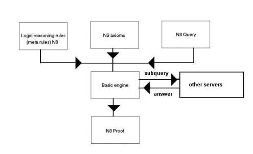
Fig.1.2. The inference engine RDFEngine in a server
with its inputs and outputs.
In fig.1.2 the global structure of the inference
engine is drawn. The inputs and outputs are in Notation 3 (N3). Notation 3 is
choosen because it is easier to work with than RDF and it is convertible to RDF
syntax. However, during the research, another syntax was developed, called
RDFProlog.
The engine is given a modular structure and different
versions exist for different testing purposes.
What has to be standardized is the input and output of
the block marked ‘Basic engine’ in fig.1.2. For the Semantic Web the precise
contents of this block will not make a part of the standard.
For making the Haskell specification the choice was made for a resolution based engine. A forward reasoning engine could have been chosen as well but a resolution based engine has better characteristics for distributed inferencing. Other choices of engine are also possible. The choice of a particular engine is not the subject of this thesis but rather the definition of the interface to the engine. However, interesting results that were obtained about resolution based inferencing are certainly worth mentioning.
1.5. The foundations
The research used mainly following material:
a) The collection of test cases of De Roo [DEROO]
b) The RDF model theory [RDFM] [RDFMS]
c) The RDF rules mail list [RDFRULES]
d) The classic resolution theory
[VANBENTHEM] [STANFORD]
e) Logic theories and mainly first order logic, constructive logic and
paraconsistent logic. [VANBENTHEM, STANFORDP]
1.6. Relation with the current research
The mail list RDF rules [RDFRULES] has as a
purpose to discuss the extension of RDF with inferencing features, mainly
rules, queries and answers. There are a lot of interesting discussions but no
clear picture is emerging at the moment.
Berners-Lee [DESIGN] seeks inspiration in first
order logic. He defines logic predicates (chapter 2), builtins, test cases and
a reference engine CWM. However the semantics of input and output formats for a
RDF engine are not clearly defined.
A common approach is to use existing logic
systems. RDF is then expressed in terms of these systems and logic (mostly
rules) is added on top e.g. Horn logic or frame logic. An example is found in
[DECKER]. In this case the semantics are those of the used logic.
The implementation of an ontology like OWL
(Ontology Web Language) implies also inferencing facilities that are necessary
for implementing the semantics of the ontology [OWL features].
Euler [DEROO] and CWM take a graph oriented
approach for the construction of the inference program. The semantics are
mostly defined by means of test cases.
The approach taken by my research for defining
the semantics of the inference input and output has two aspects:
1) It is graph oriented and, in fact, the theory is generally applicable to
labeled graphs.
2) From the logic viewpoint a constructive approach is taken for reasons of
verifiability (chapter 5).
3) A constructive graph oriented definition is given for rules, queries,
solutions and proofs.
1.7. Outline of the thesis
Chapter two gives an
introduction into the basic standards that are used by RDF and into the syntax
and model theory of RDF. Readers who are familiar with some of these matters can
skip these.
Chapter three exposes the meaning of inferencing using
an RDF facts and rules database. The Haskell specification, RDFEngine, is
explained and a theory of resolution based on reasoning on a graph is
presented.
Chapter four discusses existing software systems.
After the introduction to RDF and inferencing in chapter three, it is now
possible to highlight the most important aspects of existing softwares. The
Haskell specification RDFEngine and the theory presented in the thesis were not
based upon these softwares but upon the points mentionned in 1.5.
Chapter five explores in depth the relationship of RDF
inferencing with logic.
Here the accent is put on a constructive logic
interpretation of the graph theory exposed in chapter three.
Chapter six discusses optimalization techniques.
Especially important is a technique based on the theory exposed in chapter
three.
Chapter seven disusses inconsistencies that can arise
during the course of inferencing processes on the Semantic Web.
Chapter eight gives a brief overview of some use cases
and applications.
Chapter nine finally gives a conclusion and indicates
possible ways for further research.
Chapter 2. The building blocks
2.1.
Introduction
In this chapter a number of techniques are briefly
explained. These techniques are necessary building blocks for the Semantic Web.
They are also a necessary basis for inferencing on the web.
Readers
who are familiar with some topics can skip the relevant explanations.
2.2.XML
and namespaces
2.2.1. Definition
XML (Extensible Markup Language) is a subset of SGML (Standard General Markup
Language). In its original signification a markup language is a language which
is intended for adding information (“markup” information) to an existing
document. This information must stay
separate from the original hence the presence of separation characters. In SGML
and XML ‘tags’ are used.
2.2.2. Features
There are two kinds of tags: opening and closing tags.
The opening tags are keywords enclosed between the signs “<” and “>”. An
example: <author>. A closing tag
is practically the same, only the sign “/” is added e.g. </author>. With
these elements alone very interesting datastructures can be built. An example
of a book description:
<book>
<title>
The Semantic Web
</title>
<author>
Tim Berners-Lee
</author>
</book>
As can be seen it is quite easy to build hierarchical datastructures with these elements alone. A tag can have content too: in the example the strings “The Semantic Web” and “Tim Berners-Lee” are content. One of the good characteristics of XML is its simplicity and the ease with which parsers and other tools can be built.
The keywords in the tags can have attributes too. The
previous example could be written:
<book
title=”The Semantic Web” author=”Tim Berners-Lee”></book>
where attributes are used instead of tags.
XML is not a language but a meta-language i.e. a
language with as goal to make other languages (“markup” languages).
Everybody can make his own language using XML. A
person doing this only has to use the syntaxis of XML i.e. produce wellformed
XML. However more constraints can be added to an XML language by using DTD’s
and XML schema, thus producing valid XML documents. A valid XML document is one
that does not violate the constraints laid down in a DTD or XML schema. To
summarize: an XML language is a language that uses XML syntax and XML
semantics. The XML language can be defined using DTD’s or XML schema.
If everybody creates his own language then the
“tower-of-Babylon”-syndrome is looming. How is such a diversity in languages
handled? This is done by using namespaces.
A namespace is a reference to the definition of an XML language.
Suppose someone has
made an XML language about birds. Then he could make the following namespace
declaration in XML:
<birds:wing
xmlns:birds=”http://birdSite.com/birds/”>
This statement is referring to the tag “wing” whose description is to be found on the site that is indicated by the namespace declaration xmlns (= XML namespace). Now our hypothetical biologist might want to use an aspect of the physiology of birds described however in another namespace: <physiology:temperature xmlns:physiology=” http://physiology.com/xml/”> By the semantic definition of XML these two namespaces may be used within the same XML-object. <?xml version=”1.0” ?>
<birds:wing xmlns:birds=”http://birdSite.com/birds/”> large</birds:wing><physiology:temperature xmlns:physiology=” http://physiology.com/xml/”> 43</physiology:temperature>
2.3.URI’s and URL’s
2.3.1. Definitions
URI stands for Uniform Resource Indicator. A URI is anything that
indicates unequivocally a resource.
URL stands for Uniform Resource Locator. This is a subset of URI. A URL indicates the access to a resource. URN refers to a subset of URI and indicates names that must remain unique even when the resource ceases to be available. URN stands for Uniform Resource Name. [ADDRESSING]
In this thesis only URL’s will be used.
2.3.2. Features
The following example illustrates a URI format that is in common use.[URI]: www.math.uio.no/faq/compression-faq/part1.html Most people will recognize this as an internet address. It unequivocally identifies a web page. Another example of a URI is a ISBN number that unquivocally identifies a book.
The general format of an http URL is:
http://<host>:<port>/<path>?<searchpart>.
The host is of course the computer that contains the resource; the default port number is normally 80; eventually e.g. for security reasons it might be changed to something else; the path indicates the directory access path. The searchpart serves to pass information to a server e.g. data destinated for CGI-scripts.
When an URL finishes with a slash like http://www.test.org/definitions/ the directory definitions is addressed. This will be the directory defined by adding the standard prefix path e.g. /home/netscape to the directory name: /home/netscape/definitions.The parser can then return e.g. the contents of the directory or a message ‘no access’ or perhaps the contents of a file ‘index.html’ in that directory.
A path might include the sign “#” indicating a named anchor in an html-document. Following is the html definition of a named anchor:
<H2><A
NAME="semantic">The Semantic Web</A></H2>
A named anchor thus indicates a location within a document. The named anchor can be called e.g. by: http://www.test.org/definition/semantic.html#semantic
2.4.Resource Description Framework RDF
RDF is a language. The semantics are defined by [RDFM]; some concrete syntaxes are: XML-syntax, Notation 3, N-triples, RDFProlog. N-triples is a subset of Notation 3 and thus of RDF [RDFPRIMER]. RDFProlog is also a subset of RDF and is defined in this thesis.
Very basically RDF consist of triples: (subject, predicate, object). This simple statement however is not the whole story; nevertheless it is a good point to start.
An example [ALBANY] of a statement is:
“Jan Hanford created the J. S. Bach homepage.”.
The J.S. Bach homepage is a resource. This resource has a URI: http://www.jsbach.org/. It has a property:
creator with value ‘Jan Hanford’. Figure 2.1. gives a graphical view of this.
Creator>
</Description>
Fig.2.1. An example of a RDF relation.
In simplified RDF this is:
<RDF>
<Description about= “http://www.jsbach.org”>
<Creator>Jan Hanford</Creator>
</Description>
</RDF>
However this is without namespaces meaning that the notions are not well defined. With namespaces added this becomes:
<rdf:RDF
xmlns:rdf=”http://www.w3.org/1999/02/22-rdf-syntax-ns#”
xmlns:dc=”http://purl.org/DC/”>
<rdf:Description
about=”http://www.jsbach.org/”>
<dc:Creator>Jan
Hanford</dc:Creator>
</rdf:Description>
</rdf:RDF>
The first namespace xmlns:rdf=”http://www.w3.org/1999/02/22-rdf-syntax-ns#“
refers to the
document describing the (XML-)syntax of RDF; the second namespace xmlns:dc=”http://purl.org/DC/” refers
to the description of the Dublin Core, a basic ontology about authors and
publications. This is also an example of two languages that are mixed within an
XML-object: the RDF and the Dublin Core language.
In the
following example is shown that more than one predicate-value pair can be indicated for a resource.
<rdf:RDF
xmlns:rdf=”http://www.w3.org/1999/02/22-rdf-syntax-ns#”
xmlns:bi=”http://www.birds.org/definitions/”>
<rdf:Description
about= “http://www.birds.org/birds#swallow”>
<bi:wing>pointed</bi:wing>
<bi:habitat>forest</bi:habitat>
</rdf:Description>
</rdf:RDF>
Conclusion
What is RDF? It is a language with a simple semantics consisting of triples: (subject, predicate, object) and some other elements. Several syntaxes exist for RDF: XML, graph, Notation 3, N-triples, RDFProlog. Notwithstanding its simple structure a great deal of information can be expressed with it.
2.5.Notation 3
2.5.1. Introduction
Notation 3 is a syntax for RDF developed by Tim
Berners-Lee and Dan Connolly and represents a more human usable form of the
RDF-syntax with in principle the same semantics [RDF Primer]. Most of the test
cases used for testing RDFEngine are written in Notation 3. An alternative and
shorter name for Notation 3 is N3.
2.5.2. Basic properties
The basic
syntactical form in Notation 3 is a triple
of the form :
<subject> <verb> <object> where subject, verb and object are atoms. An atom can be either a URI (or a URI abbreviation) or a variable. But some more complex structures are possible and there also is some “ syntactic sugar”. Verb and object are also called property and value which is anyhow the semantical meaning.
In N3 URI’s can be indicated in a variety of
different ways. A URI can be indicated by its complete form or by an
abbreviation. These abbreviations have practical importance and are intensively
used in the testcases. In what follows the first item gives the complete
form; the others are abbreviations.
·
<http://www.w3.org/2000/10/swap/log#log:forAll> : this is the complete form of a URI in Notation 3. This
ressembles very much the indication of a tag in an HTML page.
·
xxx: : a label followed by a ‘:’
is a prefix. A prefix is defined in N3 by the @prefix instruction :
@prefix ont:
<http://www.daml.org/2001/03/daml-ont#>.
This defines the prefix ont: . After the label follows the URI represented by the prefix.
So ont:TransitiveProperty
is in full form <http://www.daml.org/2001/03/daml-ont#TransitiveProperty>
.
·
<#param> : Here only the tag in the HTML page is indicated. To get the complete
form the default URL must be added.the complete form is : <URL_of_current_document#param>.
The default URL is the URL of the current document i.e. the document that contains the description in Notation 3.
·
<> or <#>: this
indicates the URI of the current document.
·
: : a single double point is by convention
referring to the current document. However this is not necessarily so because
this meaning has to be declared with a prefix statement :
@prefix : <#> .
Two substantial abbreviations for sets of triples are property lists and
object lists. It can happen that a subject recieves a series of qualifications;
each qualification with a verb and an object,
e.g. :bird :color :blue;
height :high; :presence :rare.
This
represents a bird with a blue color, a high height and a rare presence.
These
properties are separated by a semicolon.
A verb or property can have several values e.g.
:bird :color :blue,
yellow, black.
This means that the bird has three colors. This
is called an object list. The two things can be combined :
:bird :color :blue,
yellow, black ; height :high ; presence :rare.
The objects in an objectlist are separated by a
comma.
A semantic and
syntactic feature are anonymous subjects.
The symbols ‘[‘ and ‘]’ are used for this feature. [:can :swim].
means there exists an anonymous subject x that can swim. The abbreviations for
propertylist and objectlist can here be used too :
[ :can :swim, :fly ; :color :yellow].
The property
rdf:type can be abbreviated as “a”:
:lion a :mammal.
really means:
:lion rdf:type :mammal.
2.6.The logic layer
In [SWAPLOG] an
experimental logic layer is defined for the Semantic Web. I will say a lot more
about logic in chapter 4. An overview of the most salient features (my engine
only uses log:implies, log:forAll, log:forSome and log:Truth):
log:implies : this is the implication, also indicated by an
arrow: à.
{:rat a :rodentia. :rodentia a :mammal.}à {:rat a :mammal}.
log:forAll : the purpose is to indicate universal variables :
{:rat a :rodentia. :rodentia a :mammal.}à {:rat a :mammal};
log:forAll :a, :b, :c.
indicates that :a, :b and :c are universal variables.
log:forSome: does the same for existential variables:
{:rat a :rodentia. :rodentia a :mammal.}à {:rat a :mammal}; log:forSome :a, :b, :c.
log:Truth : states that this is a universal truth. This is not interpreted by my engine.
Here follow briefly some other features:
log:falseHood
: to indicate that a formula is not true.
log:conjunction :
to indicate the conjunction of two formulas.
log:includes : F includes G means G follows from F.
log:notIncludes: F notIncludes G means G does not follow
from F.
2.7.Semantics
of N3
2.7.1. Introduction
The semantics of N3 are the same as the semantics of
RDF [RDFM].
The semantics indicate the correspondence between the
syntactic forms of RDF and the entities in the universum of discourse. The
semantics are expressed by a model theory. A valid triple is a triple whose elements are defined by the model
theory. A valid RDF graph is a set of
valid RDF triples.
2.7.2. The model theory of RDF
The vocabulary V
of the model is composed of a set of URI’s.
LV is
the set of literal values and XL is the mapping from the literals to LV.
A simple interpretation
I of a vocabulary V is defined by:
1. A non-empty set IR of
resources, called the domain or universe of I.
2. A mapping IEXT from IR into the powerset of IR x (IR union LV) i.e. the set of sets
of pairs <x,y> with x in IR
and y in IR or LV. This mapping
defines the properties of the RDF triples.
3. A mapping IS from V into IR
IEXT(x) is
a set of pairs which identify the arguments for which the property is true,
i.e. a binary relational extension, called the extension of x. [RDFMS]
Informally this means that every URI represents a resource which might
be a page on the internet but not necessarily: it might as well be a physical
object. A property is a relation; this relation is defined by an extension
mapping from the property into a set. This set contains pairs where the first
element of a pair represents the subject of a triple and the second element of
a pair represent the object of a triple. With this system of extension mapping
the property can be part of its own extension without causing paradoxes. This
is explained in [RDFMS].
2.7.3. Examples
Take the triple:
:bird :color :yellow.
In the set of URI’s there will be things like: :bird, :mammal, :color,
:weight, :yellow, :blue etc...These are part of the vocabulary V.
In the set IR of resources will be: #bird, #color etc.. i.e. resources
on the internet or elsewhere. #bird might represent e.g. the set of all birds.
These are the things we speak about.
There then is a mapping IEXT
from #color (resources are abbreviated) to the set
{(#bird,#blue),(#bird,#yellow),(#sun,#yellow),...}
and the mapping IS from V to
IR:
:bird à #bird, :color à #color, ...
The URI refers to a page on the internet where the domain IR is defined (and thus the semantic
interpretation of the URI).
2.8. A global view of the Semantic Web
2.8.1. Introduction.
The Semantic Web
will be composed of a series of
standards. These standards have to be organised into a certain structure that
is an expression of their interrelationships. A suitable structure is a
hierarchical, layered structure.
2.8.2. The layers of the Semantic Web
Fig.2.2. illustrates
the different parts of the Semantic Web in the vision of Tim Berners-Lee. The
notions are explained in an elementary manner here. Later some of them will be
treated more in depth.
Layer 1. Unicode and
URI
At the bottom there is Unicode and URI.
Unicode is the Universal code.
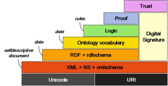
Fig.2.2. The layers
of the Semantic Web [Berners-Lee]
Unicode codes the characters of all the major languages in use today.[UNICODE].
Layer 2. XML,
namespaces and XML Schema
See 2.2. for a
description of XML.
Layer 3. RDF en
RDF Schema
The first two layers
consist of basic internet technologies. With layer 3 the Semantic Web begins.
RDF Schema (rdfs)
has as a purpose the introduction of some basic ontological notions. An example
is the definition of the notion “Class” and “subClassOf”.
Layer 4. The
ontology layer
The definitions of
rdfs are not sufficient. A more extensive ontological vocabulary is needed.
This is the task of the Web Ontology workgroup of the W3C who has defined
already OWL (Ontology Web Language) and OWL Lite (a subset of OWL).
Layer 5. The logic
layer
In the case study
the use of rules was mentioned. For expressing rules a logic layer is needed.
An experimental logic layer exists [SWAP/CWM]. This layer is treated in depth
in the following chapters.
Layer 6. The proof
layer
In the vision of Tim
Berners-Lee the production of proofs is not part of the Semantic Web. The
reason is that the production of proofs is still a very active area of research
and it is by no means possible to make a standardisation of this. A Semantic Web engine should only need to
verify proofs. Someone sends to site A a proof that he is authorised to use the
site. Then site A must be able to verify that proof. This is done by a suitable
inference engine. Three inference engines that use the rules that can be defined
with this layer are: CWM [SWAP/CWM] , Euler [DEROO] and RDFEngine developed as
part of this thesis.
Layer 7. The trust
layer
Without trust the
Semantic Web is unthinkable. If company B sends information to company A but
there is no way that A can be sure that this information really comes from B or
that B can be trusted then there remains nothing else to do but throw away that
information. The same is valid for exchange between citizens. The trust has to
be provided by a web of trust that is based on cryptographic principles. The
cryptography is necessary so that everybody can be sure that his communication
partners are who they claim to be and what they send really originates from
them. This explains the column “Digital Signature” in fig. 2.2.
The trust policy is
laid down in a “facts and rules” database. This database is used by an
inference engine like the inference engine I developed. A user defines his
policy using a GUI that produces a policy database. A policy rule might be e.g.
if the virus checker says ‘OK’ and
the format is .exe and it is signed by ‘TrustWorthy’ then accept this input.
The impression might
be created by fig. 2.2 that this whole layered building has as purpose to
implement trust on the internet. Indeed it is necessary for implementing trust
but, once the pyramid of fig. 2.2 comes into existence, on top of it all kind
of applications can be built.
Layer 8. The
applications
This layer is not in
the figure; it is the application layer that makes use of the technologies of
the underlying 7 layers. An example might be two companies A and B exchanging
information where A is placing an order with B.
Chapter 3. RDF, RDFEngine and inferencing.
3.1. Introduction
Chapter 3 will explain the meaning of
inferencing in connection with RDF. Two aspects will be interwoven: the theory
of inferencing on RDF data and the specification of an inference engine,
RDFEngine, in Haskell.
First a specification of a RDF graph will be
given. Then inferencing on a RDF graph will be explained. A definition will be
given for rules, queries, solutions and proofs. After discussing substitution
and unification, an inference step will be defined and an explanation will be
given of the data structure that is needed to perform a step. The notion of
distributed inferencing will be explained and the proof format that is
necessary for distributed inferencing.
The explanations will be illustrated with
examples and the relevant Haskell code.
RDFEngine possesses the characteristics of
monotonicity and completeness. This is demonstrated by a series of lemmas.
Note: The Haskell source code presented in the
chapter is somewhat simplified compared to the source code in appendix.
3.2.Recapitulation and definitions
I give a brief recapitulation of the most
important points about RDF [RDFM,RDF Primer, RDFSC].
RDF is a system for expressing meta-information
i.e. information that says something about other information e.g. a web page.
RDF works with triples. A triple is
composed of a subject, a property and an object. A triplelist is a
list of triples. Subject, property and object can have as value a URI, a
variable or a triplelist. An object can also be a literal. The property is also
often called predicate.
Triples are noted as: (subject, property, object). A triplelist consists of triples
between ‘[‘ and ‘]’, separated by a ‘,’.
In the graph representation subjects and
objects are nodes in the graph
and the arcs represent properties. No nodes can occur twice in the graph.
The consequence is that some triples will be connected with other triples;
other triples will have no connections. Also the graph will have different
connected subgraphs.
A node can also be an blank node which is a kind of anonymous node. A blank node can be instantiated with a URI or a literal and then becomes a ‘normal’
node.
A valid
RDF graph is a graph where all arcs are valid URI’s and all nodes are either valid URI’s, valid
literals, blank nodes or triplelists .
Fig.3.1 gives examples of triples.
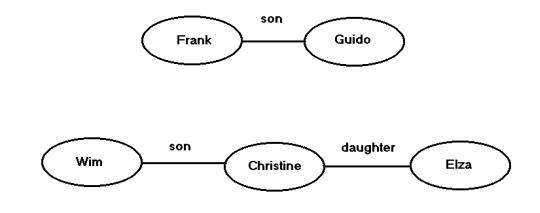
Fig.3.1.
A RDF graph consisting of two connected subgraphs.
There are three triples in the graph of fig.
3.1: (Frank, son, Guido), (Wim, son, Christine), (Christine, daughter, Elza).
I give
here the Haskell representation of triples:
data Triple = Triple (Subject,
Predicate, Object) | TripleNil
type Subject = Resource
type Predicate = Resource
type Object = Resource
data Resource = URI String |
Literal String | Var Vare | TripleList | ResNil
type TripleList1 = [Triple]
Four kinds of variables are
defined:
UVar: Universal variable with local scope
EVar: Existential variable with local scope
GVar: Universal variable with global scope
GEVar: Existential variable
with global scope
-- the definition of a variable
data Vare = UVar String | EVar
String | GVar String | GEVar String
These four kinds of variables
are necessary as they occur in the test cases of [DEROO] that were used for
testing RDFEngine.
Suppose fig.3.1 represents a RDF graph. Now
lets make two queries. Intuitively a query is an interrogation of the RDG graph
to see if certain facts are true or not.
The first query is: [(Frank,son,Guido)].
The second query is: [(?who, daughter, Elza)].
This
needs some definitions:
A query is a triplelist. The triples composing the
query can contain variables. When the query does not contain variables it is an
RDF graph. When it contains variables, it is not an RDF raph because variables
are not defined in RDF and are thus an extension to RDF. When the inferencing in RDFEngine starts the
query becomes the goallist. The
goallist is the triplelist that has to be proved i.e. matched against the RDF
graph. This process will be described in detail later.
The answer to a query consists of one or more solutions. In a solution the variables
of the query are replaced by URI’s, when the query did have variables. If not,
a solution is a confirmation that the triples of the query are existing triples
(see also 2.7). I will give later a more precise definition of solutions.
A variable
will be indicated with a question mark. For this chapter it is assumed that the
variables are local universal variables.
A grounded
triple is a triple of which subject, property and object are URI’s or literals,
but not variables. A grounded triplelist contains only grounded triples.
A query can be grounded. In that case an affirmation
is sought that the triples in the query exist, but not necessarily in the RDF
graph: they can be deduced using rules.
Fig.3.2 gives the representation of some
queries.
In the first query the question is: is Frank the son of Guido? The answer is
of course “yes”. In the second query the question is: who is a daughter of Elza?
Here the
query is a graph containing variables. This graph has to be matched with the
graph in fig.3.1. So generally for executing a RDF query what has to be done is
‘subgraph matching’.
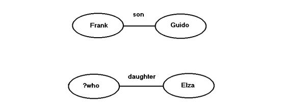
Fig.5.2.
Two RDF queries. The first query does not contain variables.
The variables in a query are replaced in the
matching process by a URI or a literal. This replacement is called a substitution. A substitution is a list
of tuples (variable, URI) or (variable, literal)[1].
The list can be empty. I will come back on substitutions later.
A rule is a triple. Its subject is a triplelist
containing the antecedents and its
object is a triplelist containing the consequents.
The property or predicate of the rule is the URI :
http://www.w3.org/2000/10/swap/log# implies. [SWAP] . I will give following
notation for a rule:
{triple1,
triple2,…} => {triple11,triple21,…}
For
clarity, only rules with one consequent will be considered. The executable
version of RDFEngine can handle multiple consequents.
For a
uniform handling of rules and other triples the concept statement is introduced in the abstract Haskell syntax:
type
Statement = (TripleList, TripleList,String)
type
Fact = Statement -- ([],Triple,String)
type
Rule = Statement
In this terminology a rule is a statement. The
first triplelist of a rule is called the antecedents
and the second triplelist is called the consequents.
A fact is a rule with empty
antecedents. The string part in the statement is the provenance information. It indicates the origin of the statement.
The origin is the namespace of the
owner of the statement.
In a rule the order of the triples is relevant.
3.3. The graph ADT
A RDF
graph is a set of statements. It is represented in Haskell by an Abstract Data Type: RDFGraph.hs.
The implementation of the ADT is done by using
an array and a hashtable.
data
RDFGraph = RDFGraph (Array Int Statement, Hash, Params)
The statements of the graph are in an array.
The elements Hash and Params in the type RDFGraph constitute a
hashtable.
A
predicate is associated with each statement. This is the predicate of the first
triple of the second triplelist of the statement1.
An entry into the hashtable has as a key a predicate name and a list of
numbers. Each number refers to an entry in the array associated with the
RDFGraph.
Params is an array containing some parameters
for the ADT like the last entry into the array of statements.
Example: Given the triple (a,b,c) that is entry number 17 in the array, the
entry in the dictionary with key ‘b’ will give a list of numbers […,17,…]. The
other numbers will be triples or rules with the same predicate.
In this way all statements with the same
associated predicate can be retrieved at once. This is used when matching
triples of the query with the RDF graph.
The ADT is accessed by means of a mini-language defined in the module
RDFML.hs. This mini-language contains functions for manipulating triples,
statements and RDF Graphs. Fig. 3.3. gives an overview of the mini-language.
Through the encapsulation by the mini-language
this implementation of the ADT could be replaced by another one where only one
module would need to be changed. For the user of the module only the
mini-language is important[2].
Mini-language for triples, statements and graphs.
--
triple :: String -> String -> String -> Triple
-- make
a triple from three strings
--
triple s p o : make a triple
nil ::
Triple
--
construct a nil triple
nil =
TripleNil
tnil ::
Triple -> Bool
-- test
if a triple is a nil triple
tnil t
| t == TripleNil = True
| otherwise = False
s ::
Triple -> Resource
-- get
the subject of a triple
s t = s1
where Triple (s1,_,_) = t
p ::
Triple -> Resource
-- get
the predicate from a triple
p t = s1
where Triple (_,s1,_) = t
o ::
Triple -> Resource
-- get
the object from a triple
o t = s1
where Triple (_,_,s1) = t
st ::
TripleSet -> TripleSet -> Statement
--
construct a statement from two triplesets
-- -1
indicates the default graph
st ts1 ts2
= (ts1,ts2,"-1")
gmpred
:: Statement -> String
-- get
the main predicate of a statement
-- This
is the predicate of the first triple of the consequents
gmpred
st
| (cons st) == [] = ""
| otherwise = pred
where t = head(cons st)
pred = grs(p t)
stnil ::
Statement
--
return a nil statement
stnil =
([],[],"0")
tstnil
:: Statement -> Bool
-- test
if the statement is a nil statement
tstnil
st
| st == ([],[],"0") = True
| otherwise = False
trule ::
Statement -> Bool
-- test
if the statement is a rule
trule
([],_,_) = False
trule st
= True
tfact ::
Statement -> Bool
-- test
if the statement st is a fact
tfact
([],_,_) = True
tfact st
= False
stf ::
TripleSet -> TripleSet -> String -> Statement
--
construct a statement where the Int indicates the specific graph.
--
command 'st' takes as default graph 0
stf ts1
ts2 s = (ts1,ts2,s)
protost
:: String -> Statement
--
transforms a predicate in RDFProlog format to a statement
-- example: "test(a,b,c)."
protost
s = st
where [(cl,_)] = clause s
(st, _, _) = transClause (cl, 1,
1, 1)
sttopro
:: Statement -> String
--
transforms a statement to a predicate in RDFProlog format
sttopro
st = toRDFProlog st
sttppro
:: Statement -> String
--
transforms a statement to a predicate in RDFProlog format with
--
provenance indication (after the slash)
sttppro
st = sttopro st ++ "/" ++ prov st
ants ::
Statement -> TripleSet
-- get
the antecedents of a statement
ants
(ts,_,_) = ts
cons :: Statement
-> TripleSet
-- get
the consequents of a statement
cons
(_,ts,_) = ts
prov ::
Statement -> String
-- get
the provenance of a statement
prov
(_,_,s) = s
fact ::
Statement -> TripleSet
-- get
the fact = consequents of a statement
fact
(_,ts,_) = ts
tvar ::
Resource -> Bool
-- test
whether this resource is a variable
tvar
(Var v) = True
tvar r =
False
tlit ::
Resource -> Bool
-- test
whether this resource is a literal
tlit
(Literal l) = True
tlit r =
False
turi ::
Resource -> Bool
-- test
whether this resource is a uri
turi
(URI r) = True
turi r =
False
grs ::
Resource -> String
-- get
the string value of this resource
grs r =
getRes r
gvar ::
Resource -> Vare
-- get
the variable from a resource
gvar (Var v) = v
graph ::
TS -> Int -> String -> RDFGraph
-- make
a numbered graph from a triple store
-- the
string indicates the graph type
-- the
predicates 'gtype' and 'gnumber' can be queried
graph ts
n s = g4
where changenr nr (ts1,ts2,_) =
(ts1,ts2,intToString nr)
g1 = getRDFGraph (map (changenr
n) ts) s
g2 = apred g1
("gtype(" ++ s ++ ").")
g3@(RDFGraph (array,d,p)) =
apred g2 ("gnumber(" ++
intToString n ++ ").")
([],tr,_) = array!1
array1 =
array//[(1,([],tr,intToString n))]
g4 = RDFGraph (array1,d,p)
agraph
:: RDFGraph -> Int -> Array Int RDFGraph -> Array Int RDFGraph
-- add a
RDF graph to an array of graphs at position n.
-- If
the place is occupied by a graph, it will be overwritten.
--
Limited to 5 graphs at the moment.
agraph g n
graphs = graphs//[(n,g)]
-- maxg defines the maximum
number of graphs
maxg :: Int
maxg = 3
statg :: RDFGraph -> TS
-- get all statements from a
graph
statg g = fromRDFGraph g
pgraph :: RDFGraph -> String
-- print a RDF graph in
RDFProlog format
pgraph g = tsToRDFProlog
(fromRDFGraph g)
pgraphn3 :: RDFGraph ->
String
-- print a RDF graph in Notation
3 format
pgraphn3 g = tsToN3
(fromRDFGraph g)
cgraph :: RDFGraph -> String
-- check a RDF graph. The string
contains first the listing of the original triple
-- store in RDF format and then
all statements grouped by predicate. The two listings
-- must be identical
cgraph g = checkGraph g
apred :: RDFGraph -> String
-> RDFGraph
-- add a predicate of arity
(length t). g is the rdfgraph, p is the
-- predicate (with ending dot).
apred g p = astg g st
where st = protost p
astg :: RDFGraph -> Statement
-> RDFGraph
-- add statement st to graph g
astg g st = putStatementInGraph
g st
dstg :: RDFGraph -> Statement
-> RDFGraph
-- delete statement st from the
graph g
dstg g st = delStFromGraph g st
gpred :: RDFGraph -> Resource
-> [Statement]
-- get the list of all
statements from graph g with predicate p
gpred g p = readPropertySet g p
gpvar :: RDFGraph ->
[Statement]
-- get the list of all
statements from graph g with a variable predicate
gpvar g = getVariablePredicates
g
gpredv :: RDFGraph ->
Resource ->[Statement]
-- get the list of all
statements from graph g with predicate p
-- and with a variable predicate.
gpredv g p = gpred g p ++ gpvar
g
checkst :: RDFGraph ->
Statement -> Bool
-- check if the statement st is
in the graph
checkst g st
| f == [] = False
| otherwise= True
where list = gpred g (p (head (cons st)))
f = [st1|st1 <- list, st1 == st]
changest :: RDFGraph ->
Statement -> Statement -> RDFGraph
-- change the value of a
statement to another statement
changest g st1 st2 = g2
where list = gpred g (p (head (cons st1)))
(f:fs) = [st|st <- list, st == st1]
g1 = dstg g f
g2 = astg g st2
setparam :: RDFGraph ->
String -> RDFGraph
-- set a parameter. The
parameter is in RDFProlog format (ending dot
-- included.) . The predicate
has only one term.
setparam g param
| fl == [] = astg g st
| otherwise = changest g f st
where st = protost param
fl = checkparam g param
(f:fs) = fl
getparam :: RDFGraph ->
String -> String
-- get a parameter. The
parameter is in RDFProlog format.
-- returns the value of the
parameter.
getparam g param
| fl == [] = ""
| otherwise = grs (o (head (cons f)))
where st = protost param
fl = checkparam g param
(f:fs) = fl
checkparam :: RDFGraph ->
String -> [Statement]
-- check if a parameter is
already defined in the graph
checkparam g param
| ll == [] = []
| otherwise = [l1]
where st = protost param
list = gpred g (p (head (cons st)))
ll = [l|l <-list, length (cons l) == 1]
(l1:ll1) = ll
assert :: RDFGraph ->
Statement -> RDFGraph
-- assert a statement
assert g st = astg g st
retract :: RDFGraph ->
Statement -> RDFGraph
-- retract a statement
retract g st = dstg g st
asspred :: RDFGraph -> String
-> RDFGraph
-- assert a predicate
asspred g p = assert g (protost
p)
retpred :: RDFGraph -> String
-> RDFGraph
--
retract a statement
retpred
g p = retract g (protost p)
Fig. 3.3. The mini-language for manipulating
triples, statements and RDF graphs.
3.4.Languages
needed for inferencing
Four languages are needed for inferencing
[HAWKE] . These languages are needed for handling:
1) facts
2) rules
3) queries
4) results
These are four data structures and using them
in inference implies using different operational procedures for each of the
languages. This is also the case in RDFEngine.
These languages can (but must not) have the
same syntax but they cannot have the same semantics. The language for facts is
based on the RDF data model. Though rules have the same representation (they
can be represented by triples and thus RDF syntax, with variables as an
extension ), their semantic interpretation is completely different from the
interpretation of facts.
The query language presented in this thesis is
a rather simple query language, for a standard engine on the World Wide Web
something more complex will be needed. Inspiration can be sought in a language
like SQL.
For representing results in this thesis a very
simple format is proposed in 3.10.
3.5.The model interpretation of a rule
A valid RDF graph is a graph where all nodes are either
blank nodes or labeled with a URI or constituted by a triplelist. All arcs are
labeled with valid URIs.
A number
of results from the RDF model theory [RDFM] are useful .
Subgraph Lemma. A graph entails1
all its subgraphs.
Instance Lemma. A graph is entailed by any of its instances.
An
instance of a graph is another graph where one or more blank nodes of the
previous graph are replaced by a URI or a literal.
Merging Lemma. The
merge2 of a set S of RDF graphs is entailed by
S and entails every member of S.
Monotonicity Lemma.
Suppose S is a subgraph of S’ and S entails E. Then S’ entails E.
These
lemmas establish the basic ways of reasoning on a graph. One basic way of
reasoning will be added: the implication. The implication, represented in
RDFEngine by a rule, is defined as follows:
Given the
presence of subgraph SG1 in graph G and the implication:
SG1 à SG2
the
subgraph SG2 is merged with G giving G’ and if G is a valid graph then G’ is a
valid graph too.
Informally,
this is the merge of a graph SG2 with the graph G giving G’ if SG1 is a
subgraph of G.
The
closure procedure used for axiomatizing RDFS in the RDF model theory [RDFM]
inspired me to give an interpetation of rules based on a closure process.
Take the following rule R describing the
transitivity of the ‘subClassOf’ relation:
{( ?c1,
subClassOf, ?c2),( ?c2, subClassOf, ?c3)} implies {(?c1,
subClassOf , ?c3)}.
The rule
is applied to all sets of triples in the graph G of the following form:
{(c1,
subClassOf, c2), (c2, subClassOf, c3)}
yielding a triple (c1, subClassOf, c3).
This last
triple is then added to the graph. This process continues till no more triples
can be added. A graph G’ is obtained called the closure of G with respect to
the rule set R1. In the ‘subClassOf’
example this leads to the transitive closure of the subclass-relation.
If a
query is posed: (cx, subClassOf, cy) then the answer is positive if this triple is
part of the closure G’; the answer is negative if it is not part of the
closure.
When variables are used in the query:
(?c1,
subClassOf, ?c2)
then the
solution consists of all triples (subgraphs) in the closure G’ with the
predicate ‘subClassOf’.
The
process of matching the antecedents of the rule R with a graph G and then
adding the consequent to the graph is called applying the rule R to the graph G.
The process is illustrated in fig. 3.4 and 3.5
with a similar example.
When more than one rule is used the closure G’ will be obtained by the repeated
application of the set of rules till no more triples are produced.
Any solution obtained by a resolution process
is then a valid solution if it is a subgraph of the closure obtained.
I will not enter into a detailed comparison
with first order resolution theory but I want to mention following point:
the
closure graph is the equivalent of a minimal Herbrand model in first order
resolution theory or a least fixpoint in fixpoint semantics.[VAN BENTHEM]
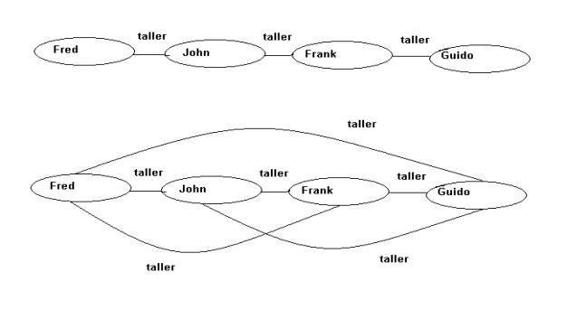
Fig.3.4.
A graph with some taller relations
and a graph representing the transitive
closure of the first graph with respect to the relation taller.
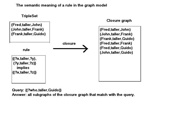
Fig. 3.5.
The closure G’ of a graph G with respect to the given rule set.
The possible answers to the query are: (Frank,taller,Guido),
(Fred,taller,Guido), (John,taller,Guido).
3.6.Unifying
two triplesets
3.6.1. Example
Fig.3.6
gives a schematic view of multiple matches of a triple with a triplelist. The
triple (Bart, son, ?w) unifies with
two triples (Bart, son, Jan) and (Bart, son, Michèle). The triple (?w, son, Paul) matches with (Guido, son, Paul) and (Jan, son, Paul). This gives 4 possible
combinations of matching triples. Following the theory of resolutions all those
combinations must be contradicted. In graph terms: they have to match with the
closure graph. However, the common variable ?w
between the first and the second triple of triple set 1 is a restriction. The
object of the first triple must be the same as the subject of the second triple
with as a consequence that there is one solution: ?w = Jan. Suppose the second
triple was: (?w1, son, Paul). Then
this restriction does not any more apply and there are 4 solutions:
{(Bart, son, Jan),(Guido, son, Paul)}
{(Bart, son, Jan), (Jan, son, Paul)}
{(Bart, son, Michèle), (Guido, son, Paul)}
{(Bart, son, Michèle), (Jan, son, Paul)}
This example shows that when unifying two triplelists the product of all the alternatives has to be taken while the substitution has to be propagated from one triple to the next for the variables that are equal and also within a triple if the same variable or node occurs twice in the same triple.
3.6.2. Definition
Let T1 and T2 be triplelists containing only
facts and T1 can contain also global, existential variables1.
Let Q be the graph represented by triplelist T1 and G the graph represented by
triplelist T2.
The unification of T1 and T2 is the set S of
subgraphs of G where each element Si of S is isomorph with a graph Q’ and each
Q’ is equal to Q with the variables of Q replaced by labels from Si.
It will
be shown that this unification can be implemented by a resolution process with
backtracking.
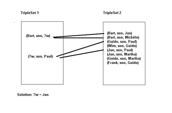 Fig.3.6.
Multiple matches within one triplelist.
Fig.3.6.
Multiple matches within one triplelist.
3.7.Unification
A triple
consists of a subject, a property and an object. Unifying two triples means
unifying the two subjects, the two properties and the two objects. A variable
unifies with a URI or a literal1. Two
URI’s unify if they are the same. The result of a unification is a
substitution. A substitution is either a list of tuples (variable, URI or
Literal). The list can be empty. The result of the unification of two triples
is a substitution (containing at most 3 tuples). Applying a substitution to a
variable in a triple means replacing the variable with the URI or literal
defined in the corresponding tuple.
type ElemSubst = (Var, Resource)
type Subst = [ElemSubst]
A nil
substitution is an empty list.
nilsub :: Subst
nilsub = []
The
unification of two statements is given in fig. 3.7.
The application
of a substitution is given in fig. 3.8.
-- appESubstR applies an
elementary substitution to a resource
appESubstR :: ElemSubst ->
Resource -> Resource
appESubstR (v1, r) v2
| (tvar v2) && (v1 == gvar v2) = r
| otherwise = v2
-- applyESubstT applies an
elementary substitution to a triple
appESubstT :: ElemSubst ->
Triple -> Triple
appESubstT es TripleNil =
TripleNil
appESubstT es t =
Triple (appESubstR es (s t), appESubstR es (p t), appESubstR es
(o t))
-- appESubstSt applies an
elementary substitution to a statement
appESubstSt :: ElemSubst ->
Statement -> Statement
appESubstSt es st = (map
(appESubstT es) (ants st),
map (appESubstT es) (cons st),
prov st)
-- appSubst applies a
substitution to a statement
appSubst :: Subst ->
Statement -> Statement
appSubst [] st = st
appSubst (x:xs) st = appSubst
xs (appESubstSt x st)
-- appSubstTS applies a substitution to a triple store
appSubstTS :: Subst -> TS
-> TS
appSubstTS subst ts = map
(appSubst subst) ts
Fig.3.7. The application of a
substitution. The Haskell source code uses the mini-language defined in
RDFML.hs
In the application of a
substitution the variables in the datastructures are replaced by resources
whenever appropriate.
3.8.Matching
two statements
The Haskell source
code in fig. 3.8. gives the unification
functions.
-- type Match = (Subst, Goals, BackStep)
-- type BackStep = (Statement, Statement)
-- unify two statements
unify :: Statement -> Statement -> Maybe
Match
-- unify two statements
unify :: Statement -> Statement -> Maybe
Match
unify st1@(_,_,s1) st2@(_,_,s2)
|
subst == [] = Nothing
|
(trule st1) && (trule st2) = Nothing
|
trule st1 = Just (subst, transTsSts (ants st1) s1, (st2,st1))
|
trule st2 = Just (subst, transTsSts
(ants st2) s2, (st2,st1))
|
otherwise = Just (subst, [stnil], (st2,st1))
where subst = unifyTsTs (cons st1) (cons st2)
-- unify two triplelists
unifyTsTs :: TripleList -> TripleList ->
Subst
unifyTsTs ts1 ts2 = concat res1
where res = elimNothing
[unifyTriples t1 t2|t1 <- ts1, t2 <-
ts2]
res1 = [sub |Just sub <- res]
unifyTriples
:: Triple -> Triple -> Maybe Subst
unifyTriples
TripleNil TripleNil = Nothing
unifyTriples t1 t2 =
if (subst1 == Nothing) || (subst2 == Nothing)
|| (subst3 ==
Nothing) then Nothing
else Just (sub1 ++ sub2 ++ sub3)
where subst1 = unifyResource (s t1) (s
t2)
subst2 = unifyResource (p t1) (p t2)
subst3 = unifyResource (o t1) (o t2)
Just sub1 = subst1
Just sub2 = subst2
Just sub3 = subst3
-- transform a tripleset to a list of statements
transTsSts :: [Triple] -> String ->
[Statement]
transTsSts ts s = [([],[t],s)|t <- ts]
unifyResource :: Resource -> Resource ->
Maybe Subst
unifyResource r1 r2
|(tvar
r1) && (tvar r2) && r1 == r2 =
Just [(gvar r1, r2)]
| tvar r1 = Just [(gvar r1, r2)]
| tvar r2 = Just [(gvar r2, r1)]
|
r1 == r1 = Just []
|
otherwise = Nothing
Fig. 3.8. The
unification of two statements
When matching a
statement with a rule, the consequents of the rule are matched with the
statement. This gives a substitution. This substitution is returned together
with the antecedents of the rule and a tuple formed by the statement and the
rule. The tuple is used for a history of the unifications and will serve to
produce a proof when a solution has been found.
The antecedents of
the rule will form new goals to be proven in the inference process.
An example:
Facts:
(Wim, brother, Frank)
(Christine, mother, Wim)
Rule:
[(?x, brother, ?y), (?z, mother, ?x)] implies
[(?z, mother, ?y)]
Query:
[(?who, mother, Frank)]
The unification of
the query with the rule gives the substitution:
[(?who, ?z), (?y, Frank)]
Following new facts
have then to be proven:
(?x, brother, Frank), (?who, mother, ?x)
(?x, brother, Frank) is unified with (Wim,
brother, Frank) giving the
substitution:
[(?x, Wim)]
and:
(?who, mother, ?x) is unified with (Christine, mother, Wim) giving the substitution:
[(?who, Christine), (?x, Wim)]
The solution then
is:
(Christine, mother, Frank).
3.9.The resolution process
RDFEngine
has been built with a standard SLD inference engine as a model: the prolog engine included in the Hugs
distribution [JONES]. The basic backtracking mechanism of RDFEngine is the
same. A resolution based inference process has three possible outcomes:
1)
it
ends giving one or more solutions
2)
it
ends without a solution
3)
it
does not end (looping state)
An
anti-looping mechanism has been provided in RDFEngine. This is the mechanism of
De Roo [DEROO].
The
resolution process starts with a query. A single query is a fact. A query can
be composed too: it then consists of more than one fact. This is equivalent to asking
more than one question. The facts of the query are entered into the goallist.
The goallist is a list of facts. A goal is selected and unified with a RDF
graph. A goal unifies with a rule when it unifies with the consequents of the
rule. The result of the unification with a rule is a substitution and a list of
goals.
A goal
can unify with many other facts or rules. Each unification will generate an alternative. An alternative consists of
a substitution and a list of goals. Each alternative will generate new
alternatives in the inference process. The graph representing all alternatives
in sequence from the start till the end of the inference process has a tree
structure1. A path from a node to a
leaf is called a search path.
When a
goal does not unify with a fact or a rule, the search path that was being
followed ends with a failure. A
search path ends with a leaf when the goallist is empty. At that point all
accumulated substitutions form a solution i.e. when these substitutions are
applied to the query, the query will become grounded.
A looping search path is an infinite
search path. An anti-looping mechanism is necessary because, if there is not
one, many queries will produce infinite search paths.
When
several alternatives are produced after a unification, one of the alternatives
will be investigated further and the others will be pushed on a stack,
together with the current substitution and the current goallist. An entry in
the stack constitutes a choicepoint.
When a search path ends in a failure, a backtrack
is done to the latest choicepoint. The goallist and the current substitution
are retrieved from the stack together with the set of alternatives. One of the
alternatives is chosen as the start of a new search path.
RDFEngine
uses a depth first search. This means that a specific search path is followed
till the end and then a backtrack is done.
In a
breadth first search for all paths one unification is done, one path after
another. All paths are thus followed at the same time till, one by one, they
reach an endpoint. In a breadth first search also an anti-looping mechanism is
necessary.
3.10.Structure of the engine
The inference engine : this is
where the resolution is executed. In RDFEngine the basic RDF data is contained
in an array of RDF graphs. The
inferencing is done using all graphs in the array.
There are three parts to RDFEngine:
a) solve : the generation of new goals by selection of a goal from the goallist
by some selection procedure1 and
unifying this goal against all statements of the array of RDF graphs thereby
producing a set of alternatives. The
process starts by adding the query to the goallist. If the goallist is empty a
solution has been found and the engine backtracks in search of other solutions.
b) choose: add new statements from one of the alternatives2 to the goallist; the other alternatives
are pushed on the stack together with the current goallist and the current
substitution. If solve did not generate any alternative goals there is a
failure (unification did not succeed) and the engine must backtrack.
c) backtrack: an alternative is retrieved from the stack together with the current
goallist and a substitution. If the stack is empty the resolution process is
finished.
An inference
step is the matching of a statement with the array of RDF graphs. An
inference step uses a data structure InfData:
data InfData = Inf
{graphs::Array Int RDFGraph, goals::Goals, stack::Stack,
lev::Level, pdata::PathData, subst::Subst,
sols::[Solution], ml::MatchList}
This data structure is specified in an Abstract
Data Structure InfADT.hs (fig.3.9). It illustrates how complex data structures
can easily be handled in Haskell using field
labels. For instance, to get access to the stack, the instruction:
stackI
= stack inf where inf
is an instance of InfData, can be
used.
This is a complex data structure. Its acess is further simplified by access routines in the ADT like e.g. sstack: show the contents of the stack in string format.
The
elements of the data structure are :
Array Int RDFGraph: The array containing the
RDF graphs.
Goals: The list of goals that
have to be proved.
Stack: The stack needed for
backtracking.
Level: The inferencing level.
This is needed for renumbering the variables and backtracking.
PathData: A list of the statements
that have been unified. This is used to establish the proof of the solutions.
Subst: The current
substitution. This substitution must be applied to the current goal.
[Solution]: The list of the
solutions.
MatchList: This is a list of Match constructors:
data Match = Match {msub::Subst, mgls::Goals,
bs::BackStep}
Matching two statements gives a
substitution, a list of goals (that may be empty) and a backstep. A backstep is nothing else than
a tuple formed by the two matched statements. This is needed for producing the
proof of a solution.
A substitution with a list of
goals forms an alternative.
An
inference step has as only input an instantiation of InfData and as only output
an instantiation of InfData. The data structure contains all the necessary
information for the next inference step.
Another
mini-language for inferencing is defined in module InfML.hs.
It is
shown in fig. 3.10.
Fig. 3.11 gives the source code of the module
that executes the inferencing process RDFEngine.hs.
data InfData = Inf {graphs::Array Int RDFGraph,
goals::Goals, stack::Stack,
lev::Level, pdata::PathData, subst::Subst,
sols::[Solution],
ml::MatchList}
* Array Int RDFGraph:
this is the array of RDF graphs
* Goals: this is the list of
goals. The format is:
type Goals = [Statement]
* Stack: the stack contains all data necessary for
backtracking. The format is:
data StackEntry = StE {sub::Subst,
fs::FactSet, sml::MatchList}
type Stack = [StackEntry]
The stack is a list of triples. The first element in the
triple is a substitution. The second element is a list of facts:
type FactSet = [Statement]
The third element is a list of matches. A match is a
triple and is the result of matching two statements:
type MatchList = [Match]
data Match = Match {msub::Subst, mgls::Goals, bs::BackStep}
Matching two statements gives a substitution, a list of
goals (that may be empty) and a backstep. A backstep is nothing else than a tuple formed by
the two matched statements:
type BackStep = (Statement, Statement)
The purpose of the backstep is to keep a history of the
unifications. This will serve for constructing the proof of a solution when it
has been found.
* Level: an integer indicating the backtacking level.
* PathData: this is a list of tuples.
data PDE = PDE {pbs::BackStep, plev::Level}
type PathData = [PDE]
The pathdata forms the history of the occurred
unifications. The level is kept also for backtracking.
* Subst:
the current substitution
*
[Solution]: the list of the
solutions. A solution is a tuple:
data Solution = Sol {ssub::Subst, cl::Closure}
A
solution is formed by a substitution and a closure. A closure is a list of
forward steps. A forward step is a tuple of statements. The closure is the
proof of the solution. It indicates how the result can be obtained with forward
reasoning. It contains the statements and the rules that have to be applied to
them.
type ForStep = (Statement,Statement)
type Closure = [ForStep]
* MatchList:
the type is explained above. The function choose needs this parameter for
selecting new goals.
3.9.
The data structure needed for performing an inference step.
Description
of the Mini Language for inferencing
For
the Haskell data types: see RDFData.hs
esub
:: Vare -> Resource -> ElemSubst (esub = elementary substitution)
esub
v t : define an elementary substitution
apps
:: Subst -> Statement -> Statement (apps = apply susbtitution)
apps
s st : apply a susbtitution to a statement
appst
:: Subst -> Triple -> Triple (appst = apply substitution (to) triple)
appst
s t : apply a substitution to a triple
appsts
:: Substitution -> TripleSet (appsts = apply substitution (to) tripleset)
appsts
s ts : apply a substitution to a tripleset
unifsts
:: Statement -> Statement -> Maybe Match (unifsts = unify statements)
unifsts
st1 st2 : unify two statements giving a match
a match is composed
of: a substitution,
the returned goals or
[], and a backstep.
gbstep
:: Match -> BackStep (gbstep = get backwards (reasoning) step
gbstep
m : get the backwards reasoning step (backstep) associated with a match.
a backstep is composed of
statement1 and statement 2 of the match
(see unifsts)
convbl
:: [BackStep] -> Substitution -> Closure (convbl = convert a backstep
list)
convbl
bl sub : convert a list of backsteps to a closure using the substitution
sub
gls
:: Match -> [Statement] (gls = goals)
gls
: get the goals associated with a match
gsub
:: Match -> Substitution (gsub = get substitution)
gsub
m : get the substitution from a match
Fig. 3.10. The mini-language for inferencing
A
process of forwards reasoning applies
rules to RDF facts deducing new facts. These facts are added to the RDF graph.
A solution is found when a graph matching of the query with the RDF graph is
possible. Either the process continues till one solution has been found, or it
continues till no more facts can be deduced.
When
RDFEngine finds a solution, the function convbl
converts a list of backsteps to a closure.
It thereby uses a substitution that is the concatenated, accumulated
substitution associated with the search path that leads to the solution. The
closure is the proof of the solution. It gives all the steps that are necessary
to deduce the solution using a forward reasoning process. The correctness of the function convbl will
be proved later.
type BackStep = (Statement, Statement)
type Closure = [ForStep]
type ForStep = (Statement, Statement)
-- convert a list of backsteps to a closure using the
substitution sub
convbl bsl sub = asubst fcl
where fcl
= reverse bsl
asubst [] = []
asubst ((st1,st2):cs) = (appSubst sub st1, appSubst sub st2):
asubst cs
--
RDFEngine version of the engine that delivers a proof
--
together with a solution
--
perform an inference step
--
The structure InfData contains everything which is needed for
-- an
inference step
infStep
:: InfData -> InfData
infStep
infdata = solve infdata
solve
inf
| goals1 == [] = backtrack inf
| otherwise = choose inf1
where goals1 = goals inf
(g:gs) = goals1
level = lev inf
graphs1 = graphs inf
matchlist = alts graphs1 level g
inf1 = inf{goals=gs,
ml=matchlist}
backtrack
inf
| stack1 == [] = inf
| otherwise = choose inf1
where stack1 = stack inf
((StE subst1 gs ms):sts) = stack1
pathdata = pdata inf
level = lev inf
newpdata = reduce pathdata
(level-1)
inf1 = inf{stack=sts,
pdata=newpdata,
lev=(level-1),
goals=gs,
subst=subst1,
ml=ms}
choose
inf
| matchlist == [] = backtrack inf
-- anti-looping controle
| ba `stepIn` pathdata = backtrack inf
| (not (fs == [])) && bool =
inf1
|
otherwise = inf2
where matchlist = ml inf
((Match subst1 fs ba):ms) =
matchlist
subst2 = subst inf
gs = goals inf
stack1 = (StE subst1 gs ms):stack
inf
(f:fss) = fs
bool = f == ([],[],"0")
pathdata = pdata inf
level = lev inf
newpdata = (PDE ba
(level+1)):pathdata
inf1 = inf{stack=stack1,
lev=(level+1),
pdata=newpdata,
subst=subst1 ++ subst2}
inf2 = inf1{goals=fs ++ gs}
--
get the alternatives, the substitutions and the backwards rule applications.
--
getMatching gets all the statements with the same property or
-- a
variable property.
alts
:: Array Int RDFGraph -> Level -> Fact -> MatchList
alts
ts n g = matching (renameSet (getMatching ts g) n) g
Fig. 3.11. The inference engine. The source code uses the mini-languages
defined in RDFML.hs, InfML.hs and RDFData.hs. The constants are mainly defined
in RDFData.hs.
3.11.The closure path.
3.11.1.Problem
In the
following paragraphs I develop a notation that enables to make a comparison
between forward reasoning (the making of a closure) and backwards reasoning
(the resolution process). The meaning of a rule and what represents a solution
to a query are defined using forward reasoning. Therefore the properties of the
backward reasoning process are proved by comparing with the forward reasoning
process.
Note:
closure path and resolution path are not paths in an RDF graph but in a search
tree.
3.11.2. The closure process
The
original graph that is given will be called G.
The closure graph resulting from the application of the set of rules will be
called G’ (see further). A rule will
be indicated by a miniscule plus an italic index. A subgraph of G or another graph (query or other) will
be indicated by a miniscule and an index.
A rule is
applied to a graph G; the antecedents
of the rule are matched with one or more subgraphs of G to yield a consequent that is added to the graph G. The consequent must be grounded for
the graph to stay a valid RDF graph. This means that the consequent can not
contain variables that are not in the antecedents.
3.11.3. Notation
A closure path is a finite sequence of
triples (not to be confused with RDF triples):
(g1,r1,c1),(g2,r2,c2), ….,(gn,rn,cn)
where (g1,r1,c1) means: the rule r1 is applied to the subgraph
(tripleset) g1 to produce
the subgraph (tripleset) c1 that is added to the graph. A closure
path represents a part of the closure process. This is not necessarily the full
closure process though the full process is represented also by a closure path.
The indices in gi,ri,ci represent sequence numbers
but not the identification of the rules and subgraphs. So e.g. r7 could be the same rule as r11.I introduce this notation
to be able to compare closure paths and resolution paths (defined further) for
which purpose I do not need to know the identification of the rules and
subgraphs.
It is
important to remark that all triples in the triplesets (subgraphs) are grounded
i.e. do not contain variables. This imposes the restriction on the rules that
the consequents may not contains variables that are absent in the antecedents.
3.11.4. Examples
In
fig.3.13 rule 1 {(?x, taller, ?y),(?y,
taller, ?z)} implies {(?x, taller, ?z)} matches with the subgraph {(John,taller,Frank),(Frank,taller,Guido)}
to
produce the subgraph {(John,taller,Guido)}
and the substitution ((x,John),(y,Frank),(z,Guido))
In the
closure process the subgraph {(John,taller,Guido)}
is added to to the original graph.
Fig. 3.12
, 3.13 and 3.14 illustrate the closure paths.
In fig.
3.19 the application of rule 1 and then rule 2
gives the closure path (I do not write completely the rules for
brevity):
({(John,taller,Frank),(Frank,taller,Guido)},rule
1, {(John,taller,Guido)}),
({(John,taller,Guido)}, rule
2,{(Guido,shorter,John)})
Two
triples are added to produce the closure graph:
(John,taller,Guido) and (Guido,shorter,John).
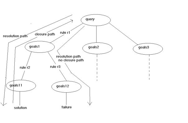
Fig.
3.12.The resolution process with indication of resolution and closure paths.
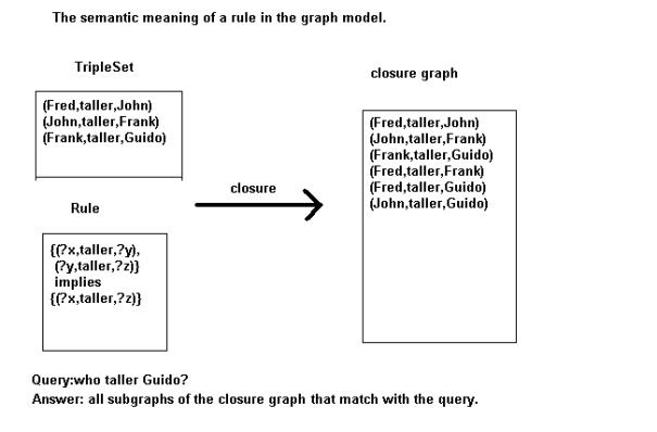
Fig.3.13. The
closure of a graph G
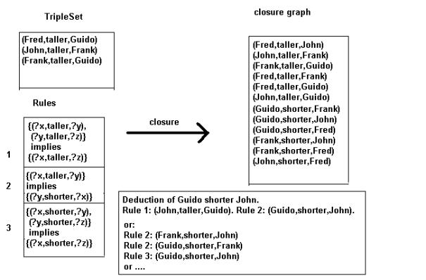
Fig.3.14. Two ways
to deduce the triple (Guido,shorter,John).
3.12.The
resolution path.
3.12.1. The process
In the resolution
process the query is unified with the database giving alternatives. An
alternative is a tripleset and a substitutionlist. One tripleset becomes a
goal. This goal is then unified etc… When a unification fails a backtrack is
done and the process restarts with a previous goal. This gives in a resolution
path a series of goals: query, goal1, goal2,… each goal being a subgraph. If
the last goal is empty then a solution has been found; the solution is a
substitutionlist. When this substitutionlist is applied to the series of goals:
query, goal1, goal2, … of the resolution
path all subgraphs in the
resolution path will be grounded i.e. they will not any more contain any
variables (otherwise the last goal cannot be empty). The reverse of such a grounded resolution path is a closure path. I will come back on this.
This is illustrated in fig. 3.12.
A subgraph g1 (a
goal) unifies with the consequents of a rule with result a substitution s and a
subgraph g1’ consisting of the antecedents of the rule
or
g1 is unified with a
connected subgraph of G with result a substitution s1 and no subgraph in
return. In this case I will assume an
identity rule has been applied i.e. a rule that transforms a subgraph into
the same subgraph with the variables instantiated. An identity rule is
indicated with rid.
The application of a
rule in the resolution process is the reverse of the application in the closure
process. In the closure process the antecedents of the rules are matched with a
subgraph and replaced with the consequents; in the resolution process the
consequents of the rule are matched with a subgraph and replaced with the
antecedents.
3.12.2. Notation
A resolution path is a finite sequence of
triples (not to be confounded with RDF triples):
(c1,r1,g1), (c2,r2,g2),
….,(cn,rn,gn)
(ci,ri,gi) means: a rule ri is applied to subgraph ci to produce subgraph gi. Contrary to what happens in a closure path gi can still contain
variables. Associated with each triple (ci,ri,gi)
is a substitution si.
The accumulated list
of substitutions [si] must
be applied to all triplesets that are part of the path. This is very important.
3.12.3. Example
An example from
fig.3.15:
The application of rule 2 to the query {(?who,shorter,John)} gives the substitution ((?x,John),(?y,Frank)) and the antecedents {(Frank,shorter,John)}.
An example of
closure path and resolution path as they were produced by a trace of the engine
can be found in annexe 2.
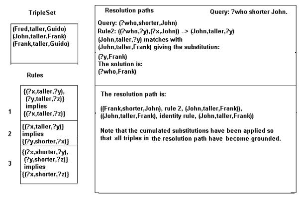
Fig.3.15. Example of a resolution path.
3.13.Variable renaming
There are two reasons why variables have to be
renamed when applying the resolution process (fig.3.16) [AIT]:
1) Different names for the variables in different rules. Though the
syntaxis permits to define the rules using the same variables the inference
process cannot work with this. Rule one might give a substitution (?x, Frank) and later on in the resolution process rule two
might give a substitution (?x,John).
So by what has ?x to be replaced?
It is possible to program the resolution process without this renaming but I think it’s a lot more complicated than renaming the variables in each rule.
2) Take the rule:
[(?x1,taller, ?y1),(?y1,taller, ?z1)]
implies [( ?x1,taller, ?z1)]
At one moment (John,taller,Fred) matches with (?x1,taller,?z1) giving substitutions:
((?x1, John),(?z1, Fred)).
Later in the process (Fred,taller,Guido) matches with (?x1,taller,?z1) giving substitutions:
((?x1, Fred),( ?z1, Guido)).
So now, by what is ?x1 replaced? Or ?z1?
This has as a consequence that the variables
must receive a level numbering where
each step in the resolution process is attributed a level number.
The substitutions above then become e.g.
((1_?x1,
John),(1_?x1, Fred))
and
((2_?x1
, Fred),(2_?z1, Guido))
This numbering is mostly done by prefixing with
a number as done above. The variables can be renumbered in the database but it
is more efficient to do it on a copy of the rule before the unification
process.
In some cases this renumbering has to be undone
e.g. when comparing goals.
The goals:
(Fred,
taller, 1_?x1).
(Fred,
taller, 2_?x1).
are really the same goals: they represent the
same query: all people shorter than Fred.
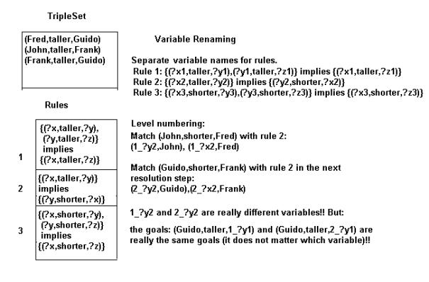
Fig.
3.16. Example of variable renaming.
3.14.Comparison of resolution and closure paths
3.14.1. Introduction
Rules,
query and solution have been defined using forward reasoning. However, this
thesis is about a backwards reasoning engine. In order then to prove the
exactness of the followed procedure the connection between backwards and
forwards reasoning must be established.
3.14.2. Elaboration
There is
clearly a likeness between closure paths and resolution paths. As well for a closure path as for a resolution
path there is a sequence of triples (x1,r1,y1) where
xi and yi are subgraphs and ri is a rule. In fact parts
of the closure process are done in reverse in the resolution process.
I want to stress
here the fact that I define closure paths and resolution paths with the complete accumulated substitution applied to
all triplesets that are part of the path.
Question: is it
possible to find criteria such that steps in the resolution process can be
judged to be valid based on (steps in ) the closure process?
If a rule is applied
in the resolution process to a triple set and one of the triples is replaced by
the antecedents then schematically:
(c, as)
where c represent
the consequent and as the antecedents.
In the closure
process there might be a step:
(as, c) where c is
generated by the subgraph as.
A closure path generates a solution when the query matches with a subgraph of the closure
produced by the closure path.
I will present some
lemmas here with explanations and afterwards I will present a complete theory.
Definitions:
A final
resolution path is the path that rests after the goallist in the (depth
first search) resolution process has been emptied. The path then consists of
all the rule applications applied during the resolution process.
A valid
resolution path is a path where the triples of the query become grounded in the
path after substitution or match with the graph G; or the resolution process
can be further applied to the path so that finally a path is obtained that
contains a solution. All resolution paths that are not valid are invalid resolution paths. The resolution
path is incomplete if after
substitution the triple sets of the path still contain variables. The
resolution path is complete when,
after substitution, all triple sets in the path are grounded.
Final Path Lemma. The
reverse of a final path is a closure path. All final paths are complete and
valid.
I will explain the
first part here and the second part later.
Take a resolution
path (q,r1,g1).
Thus the query matches once with rule r1 to generate subgraph g1
who matches with graph G. This corresponds to the closure path: (g1,r1,q ) where q in the closure G’ is generated by
rule r1.
Example: Graph G :
{(chimp, subClassOf, monkeys),( monkeys,
subClassOf, mammalia)}
And the subclassof
rule:
{(?c1, subClassOf,?c2),(?c2, subClassOf,?c3)}
implies {(?c1, subClassOf,? c3)}
- The closure
generates using the rule:
(chimp, subClassOf, mammalia)
and adds this to the database.
- The query:
{(chimp, subClassOf, ?who)}
will generate using
the rule :
{(chimp, subClassOf,?c2),(?c2, subClassOf,?c3)}
and this matches
with the database where ?c2 is substituted by monkeys and ?c3 is substituted by mammalia.
Proof:
Take the resolution
path:
(c1,r1,g1), (c2,r2,g2),
… (cn-1,rn-1,gn-1),(cn,rn,gn)
This path
corresponds to a sequence of goals in the resolution process:
c1,c2, ….,cn-1,cn. One moment or another during the process these
goals are in the goallist. Goals generate new goals or are taken from the
goallist when they are grounded. This means that if the goallist is empty all
variables must have been substituted by URI’s or literals. But perhaps a
temporary variable could exist in the sequence i.e. a variable that appears in
the antecedents of a rule x, also in the consequents of a rule y but that has
disappeared in the antecedents of rule y. However this means that there is a
variable in the consequents of rule y that is not present in the antecedents
what is not permitted.
Definition: a minimal
closure path with respect to a query is a closure path with the property
that the graph produced by the path matches with the query and that it is not
possible to diminish the length of the path i.e. to take a rule away.
Solution Lemma I: A solution corresponds to an empty closure
path (when the query matches directly with the database) or to a minimal
closure path.
Proof: This follows directly from the definition of a solution as a subgraph
of the closure graph. There are two possibilities: the triples of a solution
either belong to the graph G or are generated by the closure process. If all
triples belong to G then the closure path is empty. If not there is a closure path
that generates the triples that do not belong to G.
It is clear that
there can be more than one closure path that generates a solution. One must
only consider applying rules in a different sequence. As the reverse of the
closure path is a final resolution path it is clear that solutions can be
duplicated during the resolution process.
Solution Lemma II: be C the set of all closure paths that
generate solutions. Then there exist matching resolution paths that generate
the same solutions.
Proof: Be (g1,r1,c1),(g2,r2,c2), ….,(gn,rn,cn)
a closure path that generates a solution.
Let (cn,rn,gn),
… (c2,r2,g2),(c1,r1,g1)
be the corresponding resolution
path.
The applied rules
are called r1, r2, …, rn.
rn
applied to cn gives gn in the resolution path. Some of
the triples of gn can match with G, others will be proved by further
inferencing (for instance one of them might match with the tripleset cn-1).When
cn was generated in the closure it was deduced from gn.
The triples of gn can be part of G or they were derived with rules r1,r2,
…rn. If they were derived then the resolution process will use those
rules to inference them in the other direction. If a triple is part of G in the
resolution process it will be directly matched with a corresponding triple from
the graph G.
Final Path Lemma. The
reverse of a final path is a closure path. All final paths are complete and
valid.
I give
now the proof of the second part.
Proof: Be (cn,rn,gn),
… (c2,r2,g2),(c1,r1,g1) a final resolution path. I
already proved in the first part that it is grounded because all closure paths
are grounded. g1 is a subgraph of G (if not, the triple (c1,r1,g1) should be followed by another
one). cn is necessarily a triple of the query. The other triples of
the query match with the graph G or match with triples of ci, cj
etc.. (consequents of a rule). The reverse is a closure path. However this
closure path generates all triples of the query that did not match directly
with the graph G. Thus it generates a solution.
An
example of closure path and resolution path as they were produced by a trace of
the engine can be found in annexe 2.
3.15.Anti-looping technique
3.15.1. Introduction
The
inference engine is looping whenever
a certain subgoal keeps returning ad infinitum in the resolution process.
There are
two reasons why an anti-looping technique is needed:
1)
loopings
are inherent with recursive rules. An example of such a rule:
{(?a, subClassOf, ?b), (?b, subClassOf, ?c)}
implies {(?a, subClassOf, ?b)}
These rules occur quit often especially when
working with an ontology.
In fact, it is not even possible to seriously
test an inference engine for the Semantic Web without an anti-looping
mechanism. A lot of testcases use indeed recursive rules.
2)
an inference engine for the Semantic Web will
often have to handle rules coming from the most diverse origins. Some of these
rules can cause looping of the engine. However, because everything is meant to
be done without human intervention, looping is a bad characteristic. It is
better that the engine finishes without result, then eventually e.g. a forward
reasoning engine can be tried.
3.15.2. Elaboration
The
technique described here stems from an oral communication of De Roo [DEROO].
Given a resolution path: (cn,rn,gn),
… (c2,r2,g2),(c1,r1,g1). Suppose
the goal c2 matches with the rule r2 to generate the goal
g2. When that goal is identical to one of the goals already present
in the resolution path and generated also by the same rule then a loop may
exist where the goals will keep coming back in the path.
Take the resolution
path:
(cn,rn,gn),
…(cx,rx,gx) …(cy,ry,gy)…
(c2,r2,g2),(c1,r1,g1)
where the triples (cx,rx,gx),(cy,ry,gy)
and (c2,r2,g2) are equal
(recall that the numbers are sequence numbers and not identification numbers).
I call, by definition,
a looping path a path in which the
same triple (cx,rx,gx)
occurs twice.
The anti-looping
technique consists in failing such a path from the moment a triple (cx,rx,gx)
comes back for the second time. These triples can still contain variables so the
level numbering has to be stripped of the variables before the comparison.
No solutions are
excluded by this technique as shown by the solution lemma II. Indeed the
reverse of a looping path is not a closure path. But there exists closure paths
whose reverse is a resolution path containing a solution. So all solutions can
still be found by finding those paths.
In RDFEngine I
control whether the combination antecedents-rule returns which is sufficient
because the consequent is determined then.
In the
implementation a list of antecedents is kept. This list must keep track of the
current resolution level; when backtracking goals with higher level than the
current must be token away.
That this mechanism
stops all looping can best be shown by showing that it limits the maximum depth
of the resolution process, however without excluding solutions.
When a goal matches
with the consequent of rule r producing the antecedents as, the tuple (as, r)
is entered into a list, called the oldgoals list. Whenever this tuple (as,r)
comes back in the resolution path backtracking is done. This implies that in
the oldgoals list no duplicate entries can exist. The number of possible
entries in the list is limited to all possible combinations (as, r) that are
finite whenever the closure graph G’ is finite. Let this limit be called maxG.
Then the maximum resolution depth is maxR = maxG + maxT where maxT is the
number of grounded triples in the query and maxG are all possible combinations
(as, r). Indeed, at each step in the resolution process either a rule is used
generating a tuple (as,r) or a goal(subgraph) is matched with the graph G.
When the resolution
depth reaches maxR all possible combinations (as,r) are in the oldgoals list;
so no rule can produce anymore a couple (as,r) that is not rejected by the
anti-looping technique.
In the oldgoals list
all triples from the closure graph G’ will be present because all possible
combinations of goals and rules have been tried. This implies also that all
solutions will be found before this maximum depth is reached.
Why does this
technique not exclude solutions?
Take a closure path
(as1, r1,c1) … (asn,rn,cn)
generating a solution . No rule will be applied two times to the same subgraph
generating the same consequent to be added to the closure. Thus no asx is equal to asy. The reverse of a closure
path is a resolution path. This proofs that there exist resolution paths
generating a solution without twice generating the same tuple (as,r).
A maximal limit can
be calculated for maxG.
Be atot the total number of antecedents
generated by all rules and ntot is
the total number of labels and variables. Each antecedent is a triple and can
exist maximally in ntot**3 versions.
If there are n1 grounded
triples in the query this gives for the limit of maxG: (ntot**3) **(atot + n1).
This can easily be a
very large number and often stack overflows will occur before this number is
reached.
3.15.3.Failure
A failure (i.e. when
a goal does not unify with facts or with a rule) does never exclude solutions.
Indeed the reverse of a failure
resolution path can never be a closure path. Indeed the last triple set of
the failure path is not included in the closure. If it were its triples should
either match with a fact or with the consequent of a rule.
3.15.4.Completeness
Each solution found
in the resolution process corresponds to a resolution path. Be S the set of all
those paths. Be S1 the set of the reverse paths which are valid closure paths.
The set S will be complete when the
set S1 contains all possible closure paths generating the solution. This is the
case in a resolution process that uses depth first search as all possible
combinations of the goal with the facts and the rules of the database are
tried.
3.15.5.Monotonicity
Suppose there is a
database, a query and an answer to the query. Then another database is merged
with the first. The query is now posed again. What if the first answer is not a
part of the second answer?
In this framework
monotonicity means that when the query is posed again after the merge of
databases, the first answer will be a subset of the second answer.
The above definition
of databases, rules, solutions and queries imply monotonicity. Indeed all the
facts and rules of the first database are still present so that all the same
triples will be added during the closure process and the query will match with
the same subgraphs.
Nevertheless, some
strange results could result.
Suppose a tripleset:
{(blood,color,”red”)}
and a query:
{(blood,color,?what)}
gives the answer:
{(blood,color,”red”)}.
Now the tripleset:
{(blood,color,”yellow”)}
is added. The same
query now gives two answers:
{(blood,color,”red”)} and {(blood,color,”yellow”)}.
However this is
normal as nobody did ‘tell’ the computer that blood cannot be yellow (it could
be blue however).
To enforce this,
extensions like OWL are necessary where a restriction is put on the property
‘color’ in relation with the subject ‘blood’.
In 3.17 definitions
are given and the lemmas above and others are proved.
Fig. 3.17. gives an
overview of the lemmas and the most important points proved by them.
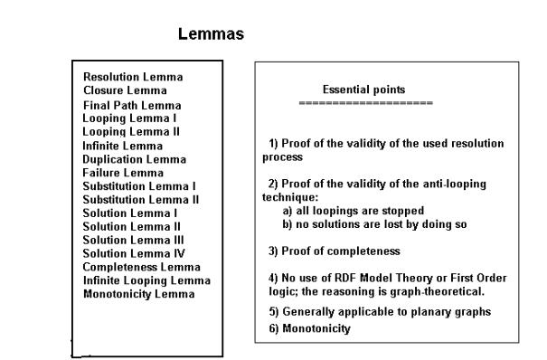
Fig.3.17. Overview
of the lemmas.
3.16.
Distributed inferencing
3.16.1. Definitions
An inference
server is a server that can accept a query and return a result. Query and result are in a standardized format.
A RDF
server is a server that can do inferencing on one or more RDF graphs. The
inferencing process uses a list of graphs. Graphs can be loaded and unloaded.
The inferencing is done over all loaded graphs.
In a process of distributed inferencing there
is a primary server and one or more secondary servers. The primary server is the server where the
inferencing process is started. The secondary servers execute part of the
inferencing process.
An
inference step is the inferencing unit
in a distributed inferencing environment. In RDFEngine an inference step
corresponds to the unification of one goal statement with the array of RDF
graphs.
3.16.2.
Mechanisms
The
program RDFEngine is organised around a basic IO loop
with the following structure:
1) Get a command from the console or a file; in automatic mode, this is a
null command.
2a) The command is independent from the
inferencing process. Execute the command. Goto 1.
2b)
read a statement from the goallist.
2)
Call
an API or execute a builtin or do an inference step.
4) Show or print results, eventually in a
trace file. Goto 1.
Fig. 3.18 gives a view of the help function.
The API permits to add builtins. Builtins are
statements with special predicates that are handled by specialized functions.
An example might be a ‘print’ predicate that performs an IO.
Example: a fact with the triplelist [(Txxx,print,”This is a message.”)].
A query can be directed to a secondary server. This is done by using
the predicate “query” in a triple (Txxx,query,”server”). This triple is
part of the antecedents of a rule. When the rule is selected the antecedents of
the rule are added to the goallist. All goals after the goal with predicate
“query” and before a goal with predicate “end_query”
will compose the distributed query. This query is sent to the secondary server
that returns a failure or a set of solutions. A solution is a substitution plus
a proof. The primary server can eventually proceed by doing a verification of
the proof. Then the returned results are added to the datastructure InfData of
the primary server who proceeds with the inference process.
Enter
command (? for help):
?
h : help
? : help
q : exit
s : perform a single inference step
g : go; stop working interactively
m : menu
e : execute menu item
qe :
enter a query Enter command (? for
help):
Fig.3.18.
The interactive interface.
This mechanism defines an interchange format between inferencing servers. The originating
server sends a query, consisting of a tripleset with existential and universal
variables. Those variables can be local (scope: one triple) or global (scope:
the whole triplelist). The secondary server returns a solution: if not empty,
it consists of the query with at least one variable substituted and of a proof.
The primary server is not concerned with what happens at the secondary server.
The secondary server does not even need to work with RDF, as long as it returns
a solution in the specified format.
Clearly, this call on a secondary server must
be done with care. In a recursive procedure this can easily lead to a kind of
spam, thereby overloading the secondary server with messages.
A possibility for reducing the traffic consists
in storing the results of the query in a rule with the format: {query}log:implies{result}. Then
whenever the query can be answered using the rule, it will not be sent anymore
to the secondary server. This constitutes a kind of learning process.
This mechanism can also be used to create virtual servers on one system, thereby
creating a modular system where each “module”
is composed of several RDF graphs. Eventually servers can be added or deleted
dynamically.
3.16.3. Conclusion
The basic IO loop
and the definition of the inferencing process on the level of one inference
step makes a highly modular structure possible. It enables also, together with
the interchange format, the possiblility to direct queries to other servers by
use of the ‘query’ and ‘end_query’ predicates.
The use of ADT’s and
mini-languages makes the program robust because changes in data structures are
encapsulated by the mini-languages.
The basic IO loop makes the program extensible by
giving the possibility of adding builtins and doing IO’s in those builtins.
3.17.A formal theory of graph resolution
3.17.1. Introduction
In this section I present more formally as a
series of definitions and lemmas what has been explained more informally in the
preceding sections.
3.17.2.Definitions
A triple consists of two labeled nodes and
a labeled arc.
A tripleset is a set of triples.
A graph is a set of triplesets.
A rule consists of antecedents and a
consequent. The antecedents are a tripleset; the consequent is a triple.
Applying a rule r to a graph G in the closure process is
the process of unifying the antecedents with all possible triples of the graph
G while propagating the substitutions. For each successful unification the
consequents of the rule is added to the graph with its variables substituted.
Applying a rule r to a subgraph g in the resolution
process is the process of unifying the consequents with all possible triples of
g while propagating the substitutions. For each successful unification the
antecedents of the rule are added to the goallist of the resolution process
(see the explanation of the resolution process).
A rule r is valid
with respect to the graph G if its closure G’ with respect to the graph G
is a valid graph.
A graph G is valid if all its elements are triples.
The graph G entails
the graph T using the rule R if T is a subgraph of the closure G’ of the graph
G with respect to the rule R.
The closure G’ of a graph G with respect to
a ruleset R is the result of the application of the rules of the ruleset R to
the graph G giving intermediate graphs Gi till no more new triples can be
generated. A graph may not contain duplicate triples.
The closure G’ of a graph G with respect to
a closure path is the resulting graph G’ consisting of G with all triples added
generated by the closure path.
A solution to a query with respect to a
graph G and a ruleset R is a subgraph of the closure G’ that unifies with the
query.
A solution set is the set of of all
possible solutions.
A closure path is a sequence of triples (gi,ri,ci)
where gi is a subgraph of a graph Gi derived from the
given graph G, ri is a rule and ci are the consequents of
the rule with the substitution si.si is the substitution
obtained trough matching a subgraph of Gi with the antecedents of
the rule ri.The tripleset ci is added to Gi to
produce the graph Gj. All triples in a closure path are grounded.
A minimal closure path with respect to a
query is a closure path with the property that the graph produced by the path
matches with the query and that it is not possible to diminish the length of
the path i.e. to take a triple away.
The graph
generated by a closure path consists of the graph G with all triples added
generated by the rules used for generating the closure path.
A closure
path generates a solution when the query matches with a
subgraph of the graph generated by the closure path.
The reverse path of a closure path (g1,r1,c1),(g2,r2,c2), ….,(gn,rn,cn) is:
(cn,rn,gn),
… (c2,r2,g2),(c1,r1,g1).
A resolution
path is a sequence of triples (ci,ri,gi)
where ci
is subgraph that matches with the consequents of the
rule ri to generate gi
and a
substitution si
. However in the resolution path the
accumulated substitutions [si]
are applied to all triplesets in the path.
A valid
resolution path is a path where the triples of the query become grounded in the
path after substitution or match with the graph G; or the resolution process
can be further applied to the path so that finally a path is obtained that
contains a solution. All resolution paths that are not valid are invalid resolution paths. The resolution
path is incomplete if after
substitution the triple sets of the path still contain variables. The
resolution path is complete when, after substitution, all triple sets in
the path are grounded.
A final
resolution path is the path that rests after the goallist in the (depth
first search) resolution process has been emptied. The path then consists of
all the rule applications applied during the resolution process.
A looping resolution path is a path with a
recurring triple in the sequence (cn,rn,gn),
…(cx,rx,gx) …(cy,ry,gy)…
(c2,r2,g2),(c1,r1,g1)
i.e. (cx,rx,gx)
is equal to some (cy,ry,gy).
The comparison is done
after stripping of the level numbering.
The resolution process is the building of
resolution paths. A depth first search
resolution process based on backtracking is explained elsewhere in the text.
3.17.3. Lemmas
Resolution Lemma. There are three possible resolution paths:
1)
a
looping path
2)
a path
that stops and generates a solution
3)
a path
that stops and is a failure
Proof. Obvious.
Closure lemma. The reverse of a closure path is a valid,
complete and final resolution path for a certain set of queries.
Proof. Take a closure path: (g1,r1,c1),(g2,r2,c2), ….,(gn,rn,cn).
This closure path adds the triplesets c1, …,cn to the
graph. All queries that match with these triples and/or triples from the graph
G will be proved by the reverse path:
(cn,rn,gn), … (c2,r2,g2),(c1,r1,g1). The reverse path is complete because all
closure paths are complete. It is final because the triple set g1 is a subgraph
of the graph G (it is the starting point of a closure path). Take now a query
as defined above: the triples of the query that are in G do of course match
directly with the graph. The other ones are consequents in the closure path and
thus also in the resolution path. So they will finally match or with other
consequents or with triples from G.
Final Path Lemma: The reverse of a final path is a closure
path. All final paths are complete and valid.
Proof:A final resolution path is the resolution path
when the goal list has been emptied and a solution has been found.
Take the resolution
path:
(c1,r1,g1), (c2,r2,g2),
… (cn-1,rn-1,gn-1),(cn,rn,gn)
This path
corresponds to a sequence of goals in the resolution process:
c1,c2, ….,cn-1,cn. One moment or another during the process these
goals are in the goallist. Goals generate new goals or are taken from the
goallist when they are grounded. This means that if the goallist is empty all
variables must have been substituted by URI’s or literals. But perhaps a
temporary variable could exist in the sequence i.e. a variable that appears in
the antecedents of a rule x, also in the consequents of a rule y but that has
disappeared in the antecedents of rule y. However this means that there is a
variable in the consequents of rule y that is not present in the antecedents
what is not permitted.
Be (cn,rn,gn),
… (c2,r2,g2),(c1,r1,g1) a final resolution path. I
already proved in the first part that it is grounded because all closure paths
are grounded. g1 is a subgraph of G (if not, the triple (c1,r1,g1) should be followed by another
one). cn matches necessarily with the query. The other triples of
the query match with the graph G or match with triples of ci, cj
etc.. (consequents of a rule). The reverse is a closure path. However this
closure path generates all triples of the query that did not match directly
with the graph G. Thus it generates a solution.
Looping Lemma I. If a looping resolution path contains a
solution, there exists another non looping resolution path that contains the
same solution.
Proof. All solutions correspond to closure paths in
the closure graph G’ (by definition). The reverse of such a closure path is
always a valid resolution path and is non-looping.
Looping Lemma II. Whenever the resolution process is looping, this is caused by a looping
path if the closure of the graph G is not infinite.
Proof. Looping means in the first place that there is
never a failure i.e. a triple or tripleset that fails to match because then the
path is a failure path and backtracking occurs. It means also triples continue
to match in an infinite series.
There are
two sublemmas here:
Sublemma 1. In a looping process at least one goal should
return in the goallist.
Proof.Can the number of goals be infinite? There is a
finite number of triples in G, a finite number of triples that can be generated
and a finite number of variables. This is the case because the closure is not
infinite. So the answer is no. Thus if the process loops (ad infinitum) there
is a goal that must return at a certain moment.
Sublemma 2. In a looping process a sequence (rule x) goal x
must return. Indeed the numbers of rules is not infinite; neither is the number
of goals; if the same goal returns infinitly, sooner or later it must return as
a deduction of the same rule x.
Infnite
Looping Path Lemma. If the closure graph G’ is
not infinite and the resolution process generates an infinite number of looping
paths then this generation will be stopped by the anti-looping technique and
the resolution process will terminate in a finite time.
Proof.
The finiteness of the closure graph implies that the
number of labels and arcs is finite too.
Suppose that a certain goal generates an
infinite number of looping paths.
This implies that the breadth of the resolution tree has to grow infinitely. It
cannot grow infinitely in one step (nor in a finite number of steps) because
each goal only generates an finite number of children (the database is not
infinite). This implies that also the
depth of the resolution tree has to grow infinitely. This implies that the level of the
resolution process grows infinitely and also then the number of entries in the
oldgoals list.
Each growth of the depth produces new entries
in the oldgoals list. (In this list each goal-rule combination is new because
when it is not, a backtrack is done by the anti-looping mechanism). In fact
with each increase in the resolution level an entry is added to the oldgoals
list.
Then at some point the list of oldgoals will
contain all possible rule-goals combinations and the further expansion is
stopped.
Formulated otherwise, for an infinite number of
looping paths to be materialized in the resolution process the oldgoals list
should grow infinitely but this is not possible.
Addendum: be maxG the maximum number of
combinations (goal, rule). Then no branch of the resolution tree will attain a
level deeper than maxG. Indeed at each increase in the level a new combination
is added to the oldgoals list.
Infinite Lemma. For a closure to generate an infinite closure
graph G’ it is necessary that at least one rule adds new labels to the
vocabulary of the graph.
Proof. Example: {:a log:math :n } à {:a
log:math :n+1). The consequent generated by this rule is each time different.
So the closure graph will be infinite. Suppose the initial graph is: :a
log:math :0. So the rule will generate the sequence of natural numbers.
If no
rule generates new labels then the number of labels and thus of arcs and nodes
in the graph is finite and so are the possible ways of combining them.
Duplication Lemma. A solution to a query can be generated by two
different valid resolution paths. It is not necessary that there is a cycle in
the graph G’.
Proof. Be (c1,r1,g1),
(c2,r2,g2), (c3,r3,g3)
and (c1,r1,g1),
(c3,r3,g3), (c2,r2,g2)
two resolution paths.Let the query q be equal to c1. Let g1 consist of c2 and
c3 and let g2 and g3 be subgraphs of G. Then both paths are final paths and
thus valid (Final Path Lemma).
Failure Lemma. If the current goal of a resolution path (the
last triple set of the path) can not be unified with a rule or facts in the
database, it can have a solution, but this solution can also be found in a
final path.
Proof. This is
the same as for the looping lemma with the addition that the reverse of a
failure path cannot be a closure path as the last triple set is not in the
graph G (otherwise there would be no failure).
Substitution Lemma I. When a variable matches with a URI
the first item in the substitution tuple needs to be the variable.
Proof. 1) The variable originates from the query.
a)
The
triple in question matches with a triple from the graph G. Obvious, because a
subgraph matching is being done.
b)
The
variable matches with a ground atom from a rule.
Suppose this happens in the resolution path when using rule r1:
(cn,rn,gn),
… (c2,r2,g2),(c1,r1,g1)
The purpose is to find a closure
path:
(g1,r1,c1),…
, (gx,rx,cx),… ,(gn, rn,cn)
where all atoms are grounded.
When rule r1 is used in
the closure the ground atom is part of the closure graph, thus in the
resolution process , in order to find a subgraph of a closure graph, the
variable has to be substituted by the ground atom.
2) A
ground atom from the query matches with a variable from a rule. Again, the
search is for a closure path that leads to a closure graph that contains the
query as a subgraph. Suppose a series of substitutions:
(v1,
a1) (v2,a2)
where a1 originates from the query corresponding to a resolution
path: (c1,r1,g1) ,(c2,r2,g2),
(c3,r3,g3).
Wherever v1 occurs it will be replaced by a1. If it
matches with another variable this variable will be replaced by a1
too. Finally it will match with a ground term from G’. This corresponds to a
closure path where in a sequence of substitutions from rules each variable
becomes replaced by a1, an atom of G’.
3) A
ground atom from a rule matches with a variable from a rule or the inverse.
These cases are exactly the same as the cases where the ground atom or the
variable originates from the query.
Substitution Lemma II. When two variables match, the variable from the
query or goal needs to be ordered first in the tuple.
Proof. In a chain of variable substitution the first
variable substitution will start with a variable from the query or a goal. The
case for a goal is similar to the case for a query. Be a series of
substitutions:
(v1,v2)
(v2,vx) … (vx,a) where a is a grounded atom.
By
applying this substitution to the resolution path all the variables will become
equal to a. This corresponds to what happens in the closure path where the
ground atom a will replace all the variables in the rules.
Solution Lemma I: A solution corresponds to an empty closure
path (when the query matches directly with the database) or to one or more minimal
closure paths.
Proof: there are two possibilities: the triples of a
solution either belong to the graph G or are generated by the closure process.
If all triples belong to G then the closure path is empty. If not there is a
closure path that generates the triples that do not belong to G.
Solution Lemma II: be C the set of all closure paths that
generate solutions. Then there exist matching resolution paths that generate
the same solutions.
Proof: Be (g1,r1,c1),…
, (gx,rx,cx),… ,(gn, rn,cn)
a closure path that generates a solution.
Let ((cn,rn,gn),
… (c2,r2,g2),(c1,r1,g1) be the corresponding resolution path.
rn applied to cn gives gn. Some of the triples of gn can match with G, others will be deduced by further
inferencing (for instance one of them might be in cn-1). When cn was generated in the closure it was deduced from gn. The triples of gn can be part of G or they
were derived with rules r1,…,
rn-2. If they were derived
then the resolution process will use those rules to inference them in the other
direction. If a triple is part of G in the resolution process it will be
directly matched with a corresponding triple from the graph G.
Solution Lemma III. The set of all valid solutions to a query q
with respect to a graph G and a ruleset R is generated by the set of all valid
resolution paths, however with elimination of duplicates.
Proof. A valid
resolution path generates a solution. Because of the completeness lemma the set
of all valid resolution paths must generate all solutions. But the duplication
lemma states that there might be duplicates.
Solution Lemma IV. A
complete resolution path generates a solution and a solution is only generated
by a complete, valid and final resolution path.
Proof. à : be (cn, rn,gn),… , (cx,rx,gx),…
, (c1,r1,g1) a complete resolution path.
If there are still triples from the query that did not become grounded by 1)
matching with a triple from G or 2) following a chain (cn, rn,gn),…, (c1,r1,g1)
where all gn match with G, the path cannot be complete. Thus all triples of
the query are matched and grounded after substitution, so a solution has been
found.
ß :
be (cn, rn,gn),…
, (cx,rx,gx),… , (c1,r1,g1) a resolution path that generates a solution.
This means all triples of the query have 1) matched with a triple from G or 2)
followed a chain (cn, rn,gn),…,
(c1,r1,g1) where gn matches with a subgraph from G. But then the
path is a final path and is thus complete (Final Path Lemma).
Completeness Lemma. The depth first search resolution process with
exclusion of invalid resolution paths generates all possible solutions to a
query q with respect to a graph G and a ruleset R.
Proof.Each solution found in the resolution process
corresponds to a closure path. Be S the set of all those paths. Be S1 the set
of the reverse paths which are resolution paths (Valid Path Lemma). The set of
paths generated by the depth first search resolution process will generate all
possible combinations of the goal with the facts and the rules of the database
thereby generating all possible final paths.
It is
understood that looping paths are stopped.
Monotonicity Lemma. Given a merge of a graph G1 with
rule set R1 with a graph G2 with rule set R2; a query Q with solution set S
obtained with graph G1 and rule set R1 and a solution set S’ obtained with
graph G2 and rule set R2. Then S is contained in S’.
Proof. Be G1’ the closure of G1. The merged graph Gm
has a rule set Rm that is the merge of rule sets R1 and R2. All possible
closure paths that produced the closure G1’ will still exist after the merge.
The closure graph G1’ will be a subgraph of the graph Gm. Then all solutions of
solution set S are still subgraphs of Gm and thus solutions when querying
against the merged graph Gm.
3.18.An extension of the theory to variable arities
3.18.1. Introduction
A RDF triple can be seen as a predicate with
arity two. The theory above was exposed for a graph that is composed of nodes
and arcs. Such a graph can be represented by triples. These are not necessarily
RDF triples. The triples consist of two node labels and an arc label. This can
be represented in predicate form where the arc label is the predicate and the
nodes are its arguments.
This theory can easily be extended to
predicates with other arities.
Such an extension does not give any more
semantic value. It does permit however to define a much more expressive syntax.
3.18.2.Definitions
A multiple of arity n is a predicate p
also called arc and (n-1) nodes also called points. The points are connected by
an (multi-headed) arc. The points and arcs are labeled and no two labels are
the same.
A graph is a set of multiples.
Arcs and
nodes are either variables or labels. (In internet terms labels could be URI’s
or literals).
Two
multiples unify when they have the same arity and their arcs
and nodes unify.
A
variable unifies with a variable or a label.
Two
labels unify if they are the same.
A rule consists of antecedents and a consequent.
Antecedents are multiples and a consequent is a multiple.
The application of a rule to a graph G consists in unifying the
antecedents with multiples from the graph and, if successful, adding the
consequent to the graph.
3.18.3. Elaboration
The
lemmas of the theory explained above can be used if it is possible to reduce
all multiples to triples and then proof that the solutions stay the same.
Reduction of multiples to triples:
Unary
multiple: In a graph G a becomes (a,a, a) .In a query a becomes (a,a,a). These
two clearly match.
Binary
multiple: (p,a) becomes (a,p,a). The
query (?p,?a) corresponds with (?a, ?p, ?a).
Ternary
multiple: this is a triple.
Quaternary
multiple: (p, a, b, c) becomes:
{(x, p,
a), (x, p, b), (x,p,c)} where x is a unique temporary label.
The query
(?p,?a,?b,?c) becomes:
{(y,?p,?a),(y,?p,?b),(y,?p,?c)}.
It is quit obvious
that this transformation does not change the solutions.
Other arities are
reduced in the same way as the quaternary multiple.
3.19.An
extension of the theory to typed nodes and arcs
3.19.1. Introduction
As argued also
elsewhere (chapter 6) attributing types to the different syntactic entities
i.e. nodes and arcs could greatly facilitate the resolution process. Matchings
of variables with nodes or arcs that lead to failure because the type is not
the same can thus be impeded.
3.19.2. Definitions
A sentence is a sequence of syntactic
entities. A syntactic entity has a type
and a label. Example:
verb/walk.
Examples
of syntactic entities: verb, noun, article, etc… A syntactic entity can also be a variable. It is then preceded by an
interrogation mark.
A language is a set of sentences.
Two sentences unify if their entities unify.
A rule consists of antecedents that are
sentences and a consequent that is a sentence.
3.19.3. Elaboration
An example:
{(noun/?noun, verb/walks)} à {(article/?article,noun/ ?noun, verb/walks)}
In fact what is done
here is to create multiples where each label is tagged with a type. Unification
can only happen when the types of a node or arc are equal besides the label
being equal.
Of course sentences
are multiples and can be transformed to triples.
Thus all the lemmas
from above apply to these structures if solutions can be defined to be
subgraphs of a closure graph. .
This can be used to
make transformations e.g.
(?ty/label,object/?ty1)
à (par/’(‘, object/?ty1).
Parsing can be done:
(?/charIn
?/= ?/‘(‘) à
(?/charOut ?/= par/’(‘)
Chapter 4. Existing software systems
4.1. Introduction
After discussing the characteristics of RDF
inferencing it is possible to review existing softwares.
I make a difference between a query
engine that just does querying on a RDF graph but does not handle rules and
an inference engine that also handles
rules.
In the literature this difference is not always so clear.
The complexity of an inference engine is a lot higher than a query engine. This is because rules create an extension of the original graph producing a closure graph (see chapter 3). In the course of a query this closure graph or part of it has to be reconstructed. This is not necessary in the case of a query engine.
Rules also suppose a logic base that is inherently more complex than the logic in the situation without rules. For a query engine only the simple principles of entailment on graphs are necessary (see chapter 3).
RuleML is an important effort to define rules that are usable for the World Wide Web [GROSOP].
The Inference Web [MCGUINESS2003] is a recent realisation that defines a system for handling different inferencing engines on the Semantic Web.
4.2. Inference engines
4.2.1.Euler
Euler is the program made by Deroo [DEROO]. It does inferencing and also implements a great deal of OWL (Ontology Web Language).
The program reads one or more triple databases that are merged together and it also reads a query file. The merged databases are transformed into a linked structure (Java objects that point to other Java objects). The philosopy of Euler is thus graph oriented.
This structure is different from the structure of RDFEngine. In my engine the graph is not described by a linked structure but by a collection of triples, a tripleset.
The internal mechanism of Euler is in accordance with the principles exposed in chapter 3.
Deroo also made a collection of test cases upon which I based myself for testing RDFEngine.
4.2.2. CWM
CWM is the program of Berners-Lee.
It is based on forward reasoning.
CWM makes a difference between existential and
universal variables[BERNERS]. RDFEngine does not make that difference. It
follows the syntaxis of Notation 3: log:forSome
for existential variables, log:forAll for universal variables. As will be explained
in chapter 6 all variables in my engine are quantified in the sense: forAllThoseKnown. Blank or anonymous
nodes are instantiated with a unique URI.
CWM makes a difference between ?a for a universal, local variable and _:a for an existential, global variable. RDFEngine maintains the
difference between local and global but not the quantification.
4.2.3. TRIPLE
TRIPLE is
based on Horn logic and borrows many features from F-Logic [SINTEK].
TRIPLE is the successor of SiLRI.
4.3. RuleML
4.3.1. Introduction
RuleML is an effort to define a specification of rules for use in the World Wide Web.
4.3.2. Technical approach
The kernel of RuleML are datalog logic programs (see chapter 6) [GROSOF]. It is a declarative logic programming language with model-theoretic semantics. The logic is based on Horn logic.
It is a webized language: namespaces or defined as well as URI’s.
Inference engines are available.
There is a cooperation between the RuleML Iniative and the Java Rule Engines Effort.
4.4. The Inference Web
4.4.1. Introduction
The Inference Web was introduced by a series of recent articles [MCGUINESS2003].
When the
Semantic Web develops it is to be expected that a variety of inference engines
will be used on the web. A software system is needed to ensure the
compatibility between these engines.
The inference web is a software system consisting of:
a web based registry containing details on information sources and reasoners called the Inference Web Registry.
1) an interface for entering information in the registry called the Inference Web Registrar.
2) a portable proof specification
3) an explanation browser.
4.4.2. Details
In the Inference Web Registry data about inference engines are stored. These data contain details about authoritative sources, ontologies, inference engines and inference rules. In the explanation of a proof every inference step should have a link to at least one inference engine.
1) The
Web Registrar is an interface for entering information into the Inference Web
Registry.
2) The
portable proof specification is written in the language DAML+OIL. In the future
it will be possible to use OWL. There
are four major components of a portable proof:
a) inference
rules
b) inference
steps
c) well
formed formulae
d) referenced
ontologies
These are the components of the inference process and thus produces the
proof of the conlusion reached by the inferencing.
3) The
explanation browser show a proof and permits to focus on details, ask
additional information, etc…
4.4.3. Conclusion
I believe the Inference Web is a major and important step in the development of the Semantic Web. It has the potential of allowing a cooperation between different inference engines. It can play an important part in establishing trust by giving explanations about results obtained with inferencing.
4.5. Query engines
4.5.1. Introduction
RDFEngine uses
rather simple query expressions: they are just subgraphs. Many RDF query
engines exists that use much more sophisticated query languages. Many of these
have been inspired by SQL [RQL].
Besides giving a subgraph as a query, many other extra features are
often implemented. E.g. for queries that result in an answer containing
mathematical values, certain boundaries can be imposed on the resulting query.
There are many RDF
query engines. I will only discuss some of the most important.
4.5.2. DQL
DAML Query Language (DQL) is a formal language and
protocol for a querying agent and an answering agent to use in conducting a query-answering dialogue using knowledge
represented in DAML+Oil.
The DQL
specification [DQL] contains some interesting notions:
a)
variables in a
query can be: must-bind, may-bind or don’t-bind. Must-bind variables must be
bound to a resource. May-bind variables may be bound. Don’t-bind variables may
not be bound.
b)
The set of all
answers to a query is called the response
set. In general, answers will be delivered in group, each of which is
called an answer bundle. An answer
bundle contains a server continuation
that is either a process handle that
can be used to get the next answer bundle or a termination token indicating the end of the response.
4.5.3. RQL
RQL uses a SQL-like syntax for querying. Following
features are worth mentioning:
a) RDF
Schema is built-in. Class-instance relationships, classe/property subsumption,
domain/range and such are adressed by specific language constructs [RQL]. This means that the query engine does
inferencing. It will e.g. deduce all classes a resource belongs to by following
the subclass relationships.
b) RQL has operators: comparison and
logical operators.
c) RQL has set operations: union, intersection and difference.
An example:
select
X, Y
from
{X : cult:cubist } cult:paints {Y}
using
namespace
cult = http://www.icom.com/schema.rdf#
The query asks for the paintings of all painters who are cubists.
4.5.4. XQuery
XQuery is a programming language[BOTHNER]. Everything in XQuery is an expression which evaluates to a value. Some characteristics are:
1) The primitive data types in Xquery are the same as for XML Schema.
2) XQuery can represent XML values. Such values are: element, attribute, namespace, text, comment, processing-instruction and document.
3) XQuery expressions evaluate to sequences of simple values.
4) XQuery borrows path expressions from Xpath. A path expression indicates the location of a node in a XML tree.
5) Iterating over sequences is possible in XQuery (see the example).
6) It is possible to define functions in XQuery.
7) Everything reminds of functional programming.
Example:
for $c
in customers
for $o
in orders
where
$c.cust_id=$o.cust_id and $o.part_id="xx"
return
$c.name
This corresponds to following SQL statements:
select customers.namefrom customers, orderswhere customers.cust_id=orders.cust_id and orders.part_id="xx"In Haskell this could be represented by following list comprehension:[name c| c <- customers, o <- orders, cust_id c == cust_id1 o, part_id o == “xx”]
4.6. Swish
Swish is a software
package that is intended to provide a framework for building programs in
Haskell that perform inference on RDF data [KLYNE]. Where RDFEngine uses
resolution backtracking for comparing graphs, Swish uses a graph matching
algorithm described in [CARROLL]. This algorithm is interesting because it
represents an alternative general way, besides forwards and backwards
reasoning, for building a RDF inference engine.
Chapter
5. RDF, inferencing and logic.
5.1.The
model mismatch
When the necessity was felt to define
rules as a layer above RDF and rdfs inspiration was sought in the beginning
with first order logic (FOL) and more specifically with horn clauses.[SWAP,
DECKER, RDFRULES]. Nevertheless the model theory of RDF is completely graph
oriented. This creates a model mismatch
where on the one hand a graph model and entailment on graphs is followed when
using basic RDF, on the other hand FOL reasoning is followed when using
inferencing.
This raises the
question: how do you translate between the two models or is this even possible?
Indeed, the
semantics of the graph model and those of first order logic are not the same.
There are points of
difference between the graph model of RDF and FOL:
1)
RDF only uses the
logic ‘and’ by way of the implicit
conjunction of RDF triples. The logic layer adds the logic implication and
variables. Negation and disjunction (or), where necessary, have to be
implemented as properties of subjects. The implication as defined for RDF is
usually not the same as the first order material implication.
2)
Is a FOL predicate the same as an RDF
property? Is a predicate
Triple(subject,property,object) really the same as a triple (subject,property, object)?
3)
The quantifiers
(forAll, forSome) are not really ‘existing’. A solution is a match of a query
with the closure graph. The quantifier used is then: ‘for_all_known_in_our_database’. The database can be an ad-hoc
database that came to existence by a merge of several RDF-databases.
4)
The logic as
defined in the preceding chapter is not the same as FOL. This will be discussed
more in depth in the following. As an example lets take the implication: a à b in FOL implies Øb à Øa in FOL. This is not true for the rules defined
in the preceding chapter:
(s1,p1,o1)implies(s2,p2,o2) does not imply (not(s2,p2,o2))implies (not(s1,p1,o1)). This not is not even defined!
I have made a model of RDF in FOL without however
claiming the isomorphism of the translation. Others have done the same before
[RDFRULES]. In this model RDF and the logic extension are both viewed in terms
of FOL and the corresponding resolution theory.
I have constructed also a model of RDF and the logic
layer with reasoning on graphs (chapter 3). Here the compatibility with the RDF
model theory is certain. The model enabled me to prove some characteristics of
the resolution process used for the Haskell engine, RDFEngine.
5.2.Modelling
RDF in FOL
5.2.1. Introduction
RDF works with triples. A triple is composed of a
subject, predicate and object. These items belong together and may not be
separated. To model them in FOL a predicate Triple can be used :
Triple(subject,
predicate, object)
Following the model theory [RDFM] there can be sets of
triples that belong together. If t1, t2 and t3 are triples, a set of triples
might be modelled as follows:
Tripleset(t1,
t2, t3)
This is however not correct as the length of the set is variable; so a list must be used.
There exist also anonymous subjects: these can be
modelled by an existential variable:
$ X: Triple(X, b, c)
saying that there exists something with property b and
value c.
An existential elimination can also be applied putting
some instance for the variable (existential elimination):
Triple(_ux,
b, c)
5.2.2. The RDF data model
Now let's consider the RDF data model [RDFM]: fig.
5.1.
Note: for convenience Triple will be abbreviated
T and Tripleset TS.
This datamodel gives the first order facts and
rules as shown in fig. 5.2.
(a set is represented by rdfs:Class).
As subjects and objects are Resources they can
be triples too (called “embedded triples”); predicates however cannot be
triples because of rule 6. This can be used for an important optimization in
the unification process.
Reification of a triple {pred, sub, obj} [RDFM] of Statements is an element r of Resources representing the reified triple and the elements s1, s2, s3, and s4 of Statements such that :
The RDF data model
Point 1-4 describe the sets in the model :
1) There is a set called Resources.
2) There is a set called Literals.
3) There is a subset of Resources called Properties.
4) There is a set called Statements, each element of which is a triple
of the form
{pred, sub, obj}
where pred is a property (member of Properties), sub is a resource
(member of Resources), and obj is either a resource or a literal (member of
Literals).(Note: this text will use the sequence {sub, pred, obj}).
The following points give extra properties:
5)RDF:type is a member of Properties.
6)RDF:Statement is a member of resources but not contained in
Properties.
7)RDF:subject, RDF:predicate and RDF:object are in Properties.
Fig. 5.1.
The RDF data model.
The
RDF data model in First Order Logic
1)
T(rdf:Resources, rdf:type, rdfs:Class)
2)
T(rdf:Literals, rdf:type, rdfs:Class)
3)
T(rdf:Resources, rdfs:subClassOf,
rdf:Properties)
4)
T(rdf:Statements, rdf:type, rdfs:Class)
"s,
sub, pred, obj: T(s, rdf:type, rdf:Statements) à (Equal(s, Triple(sub, pred, obj)) Ù
T(pred, rdf:type, rdf:Property) Ù
T(sub, rdf:type, rdf:Resources) Ù
T(obj, rdf:type, rdf:Resources) Ú
T(obj, rdf:type, rdf:Literals)))
5)
T(rdf:type, rdf:type, rdf:Property) Note the recursion here.
6)
T(rdf:Statement, rdf:type, rdf:Resources)
ØT(rdf:Statement,
rdf:type, rdf:Property)
7)
T(rdf:subject, rdf:type, rdf:Property)
T(rdf:predicate, rdf:type, rdf:Property)
T(rdf:object, rdf:type, rdf:Property)
Fig. 5.2. The RDF data model in First Order
Logic
s1: {RDF:predicate, r, pred}
s2: {RDF:subject, r, subj}
s3: {RDF:object, r, obj}
s4: {RDF:type, r, RDF:Statement}
In FOL:
"r, sub, pred, obj: T(r, rdf:type, rdf:Resources) Ù T(r, rdf :predicate, pred) Ù T(r, rdf:subject, subj) Ù T(r, rdf:subject, obj) -> T(r, Reification, T(sub, pred, obj))
The property ‘Reification’ is introduced here.
As was said a set of triples has to be represented by a list:
If T(d,e,f),
T(g,h,i) and T(a,b,c) are triples
then the list of this triples is :
{:d
:e :f. :g :h :i. :a :b :c} becomes:
TS(T(d,
e, f),TS(T(g,h,i),TS(T(a,b,c))))
In prolog e.g. :
[T(d,
e, f)|T(g, h, i)|T(a, b, c].
In Haskell this is better structured:
type
TripleSet = [Triple]
tripleset
= [Triple(d, e, f), Triple(g, h, i),
Triple(a, b, c)]
5.2.3. A problem with reification
Following the data
model a node in the RDF graph can be a triple. Such a node can be serialised
i.e. the triple representing the node is given a name and then represented
separately by its name.
Example: T(Lois,believes,T(Superman,capable,fly)).
[Sabin]
This triple expresses a so called quotation. It is not the intention that
such a triple is asserted i.e. considered to be true.
So, given the triple: T(Superman,identical,ClarkKent) it should not be infered:
T(Lois,believes,T(ClarkKent,capable,fly)).
The triple T(Lois,believes,T(Superman,capable,fly)). should be serialised as follows:
T(Lois,believes,t).
T(RDF:predicate, t, capable).
T(RDF:subject, t, Superman).
T(RDF:object, t, fly).
T(RDF:type, t, RDF:Statement).
The reified triples do not belong to the same RDF graph as the triple:
T(Lois,believes,T(Superman,capable,fly)) as can easily be verified.
The triple T(Superman,identical,ClarkKent)
can not be unified with this reification.
The conclusion is that separate triples should
not be unified with embedded triples i.e. with triples that represent a node in
the RDF graph. The possibility of representing nodes by a triples or a
tripleset enhances considerably the expressiveness of RDF as I have been able
to conclude from some experiments.
However the data model states:
RDF:Statement
is a member of resources but not contained in Properties.
Strictly speaking then one triple can compose a node but not a tripleset. Nevertheless, I’m in favour of permitting a resource to be constituted by a tripleset.
Consider now the Notation3 statement:
:Lois
:believes {:Superman :capable :fly}.
Now this
can be interpreted in two ways (with a different semantic interpretation):
1) :Lois :believes :Superman.
:Superman :capable :fly.
Here
however the ‘quoting’ aspect has vanished.
2) The
second interpretation is by reification as above.
I will
take it that the second interpretation is the right one.
Klyne [Klyne2002] gives also an analysis of
these embedded triples also called formulae.
5.2.4.Conclusion
The RDF data model can be reduced to a subset of first
order logic. It is restricted to the use of a single predicate Triple and lists
of triples. However this model says nothing about the graph structure of RDF.(See
chapter 3).
For convenience in what follows lists will be
represented between ‘[]’; variables will be identifiers prefixed with ?.
5.3.Unification
and the RDF graph model
An RDF graph is a set of zero, one or more connected
subgraphs. The elements of the graph are subjects, objects or bNodes (=
anonymous subjects). The arcs between the nodes represent predicates.
Suppose there is the following database:
TS[T(Jack,
owner, dog),T(dog, name, “Pretty”), T(Jack, age, “45”)]
And a query: TS(T(?who,
owner, dog), T(dog, name, ?what))
If we represent the first subgraph of the database and
the first query as follows:
T(Jack, owner, dog)
Ù T(dog, name, “Pretty) Ù T(Jack, age, “45”)
and the query(here negated for the proof):
ØT(?who,
owner, dog) Ú ØT(dog,
name, ?what)
Then by applying the rule of UR (Unit Resolution) to the query and the triples T(Jack, owner, dog) and T(dog, name, “Pretty) the result is the substitution: [(?who, Jack),(?what, “Pretty”)] .
Proof of this application: T(a) Ù T(b) Ù (ØT(a) Ú ØT(b)) =
T(a)
Ù (T(b) Ù ØT(a)) Ú (T(b) Ù ØT(b)) = T(a) Ù (T(b) Ù ØT(a)) = False
This proof can be
extended to any number of triples. This is in fact UR resolution with a third
empty clause.
In [WOS]: “Formally,
UR-resolution, is that inference rule that applies to a set of clauses one of
which must be a non-unit clause, the remaining must be unit clauses, and the
result of successful application must be a unit clause. Furthermore, the
nonunit clause must contain exactly one more literal than the number of (not
necessarily distinct) unit clauses in the set to which UR-resolution is being
applied.“
An example of
UR-resolution(in prolog style):
rich(John) Ú happy(John) Ú tall(John)
Ørich(John)
Øhappy(John)
tall(John)
A query (goal)
applied to a rule gives:
(T(a) Ù T(b)) à T(c) = Ø T(a) Ú
Ø T(b) Ú T(c)
where the query will
be : Ø T(?c)
Here the application
of binary resolution gives the new goal:
Ø T(a) Ú Ø T(b) and the substitution (?c, c).
In [WOS] : “ Formally, binary
resolution is that inference rule that takes two clauses, selects a literal in
each of the same predicate but of opposite sign, and yields a clause providing
that the two selected literals unify. The result of a successful application of
binary resolution is obtained by applying the replacement that unification
finds to the two clauses, deleting from each (only) the descendant of the
selected literal, and taking the or of
the remaining literals of the two clauses. “
An example (in prolog style) of binary resolution:
rich(John)
Ú
happy(John)
Ørich(John) Ú tall(John)
happy(John)
Ú tall(John)
This application does not produce a contradiction; it
adds the clause Ø T(a) Ú Ø T(b) to the goallist.
The logical implication is not part of RDF or RDFS. It will be part of a logic standard for the Semantic Web yet to be established.
This unification mechanism is classical FOL
resolution.
5.4.Completeness
and soundness of the engine
The algorithm used
in the engine is a resolution algorithm. Solutions are searched by starting
with the axiom file and the negation of the lemma (query). When a solution is
found a constructive proof of the lemma has also been found in the form of a
contradiction that follows from a certain number of traceable unification steps
as defined by the theory for first order resolution. Thus the soundness of the
engine can be concluded.
In general completeness of a RDF engine is not necessary or even possible. It can be possible for subsets of RDF and, for certain applications, it might be necessary. It is an engine for verification of proofs; no assurance can be given if a certain proof is refused about the validity of the proof. If it is accepted the garantuee is given of its correctness.
The
unification algorithm clearly is decidable as a consequence of the simple
ternary structure of N3 triples. The unification algorithm in the module
RDFUnify.hs can be seen as a proof of this.
5.5.RDFProlog
I have defined a prolog-like structure by the module RDFProlog.hs (for a sample see chapter 9. Applications) where e.g. name(company,”Test”) is translated to the triple: (company,name,”Test”). This language is very similar to the language DATALOG that is used for a deductive access to relational databases [ALVES].
The alphabet of DATALOG is composed of three sets: VAR,CONST and PRED
denoting respectively variables, constants and predicates. One notes the absence of functions. Also predicates are not nested.
In RDFProlog the general format of a rule is:
predicate-1(subject-1,object-1),…,
predicate-n(subject-n,object-n) :>
predicate-q(subject-q,object-q),
…,predicate-z(subject-z,object-z).
where all predicates,subjects and objects can be variables.
The format of a fact is:
predicate-1(subject-1,object-1),…,
predicate-n(subject-n,object-n).
where all predicates,subjects and objects can be variables.
This is a rule without antecedents.
Variables begin with capital letters.
All clauses are to be entered on one line. A line with a syntax error is neglected. This can be used to add comment.
The parser is taken from [JONES] with minor modifications.
5.6.From Horn clauses to RDF
5.6.1. Introduction
Doubts have often
been uttered concerning the expressivity of RDF. An inference engine for the
World Wide Web should have a certain degree of expressiveness because it can be
expected, as shown in chapter one, that the degree of complexity of the
applications could be high.
I will show in the next section that all Horn clauses
can be transformed to RDF, perhaps with the exeception of functions. This means
that RDF has at least the same expressiveness as Horn clauses.
5.6.2. Elaboration
For Horn clauses I will use the Prolog syntax; for RDF
I will use Notation 3.
I will discuss this by giving examples that can be
easily generalized.
0-ary predicates:
Prolog: Venus.
RDF: [:Tx
:Venus] or :Ty :Tx :Venus.
where
:Ty and :Tx are created anonymous URI’s.
Unary predicates:
Prolog: Name(“John”).
RDF: [:Name
“John”] or :Ty :Name “John”.
Binary predicates:
Prolog: Author(book1,
author1).
RDF: :book1
:Author :author1.
Ternary and higher:
Prolog: Sum(a,b,c).
RDF: :Ty
:Sum1 :a.
:Ty :Sum2 :b.
:Ty :Sum3 :c.
where :Ty represents the sum.
Embedded predicates: I will give an extensive example.
In Prolog:
diff(plus(A,B),X,plus(DA,DB)) :-
diff(A,X,DA), diff(B,X,DB).
diff(5X,X,5).
diff(3X,X,3).
and the query:
diff(plus(5X ,3X),X,Y).
The solution is: Y
= 8.
This can be put in RDF but the source is rather more verbose. The result is given in fig. 5.3. Comment is preceded by #.
This is really very verbose but... it can be automated
and it does not necessarily have to be less efficient because special measures
are possible for enhancing the efficiency due to the simplicity of the format.
So the thing to do with embedded predicates is to externalize
them i.e. to make a separate predicate.
What remains are functions:
Prolog: p(f(x),g).
RDF: :Tx :f :x.
:Tx
:p :g.
or first: replace p(f(x),g)
with p(f,x,g) and then proceed as
before.
Hayes in [RDFRULES] warns however that this way of replacing
a function with a relation can cause problems when the specific aspects of a
function are used i.e. when only one value is needed.
5.7. Comparison with Prolog and Otter
5.7.1. Comparison of Prolog with RDFProlog
Differences between Prolog and RDFProlog are:
1) predicates can be variables in RDFProlog:
P(A,B),P(B,C) :> P(A,C).
This is not permitted in Prolog.
These difference is not very fundamental as anyhow using this feature does not produce very good programs. Especially this point can very easily lead to combinatorial explosion.
The RDF Graph:
{?y1 :diff1 ?A.
?y1 :diff2
?X.
?y1 :diff3 ?DA. # diff(A,X,DA)
?y2 :diff1 ?B.
?y2 :diff2
?X.
?y2 :diff3
?DB. # diff(B,X,DB)
?y3 :plus1 ?A.
?y3
:plus2 ?B. # plus(A,B)
?y4 :diff1 ?y3.
?y4 :diff2
?X. #diff(plus(A,B),X,
?y5 :plus1 ?DA.
?y5
:plus2 ?DB.} # plus(DA,DB)
log:implies{
?y4 :diff3
?y5.}. # ,plus(DA,DB)) -- This was the rule part.
:T1 :diff1 :5X. # here starts the data part
:T1 :diff2 :X.
:T1 :diff3
:5. # diff(5X,X,5).
:T2 :diff1
:3X.
:T2 :diff2
:X.
:T2 :diff3
:3. # diff(3X,X,3).
:T4 :plus1 :5X.
:T4 :plus2 :3X. # plus(5X,3X).
:T5 :diff1 :T4.
:T5 :diff2 :X. # diff(T4,X,
:T6 :plus1 :5.
:T6 :plus2 :3. # plus(5,3)
The query:
:T5 :diff3 ?w. #
,Y))
The answer:
:T5
:diff3 :T6.
Fig. 5.3. A differentiation in RDF.
2) RDFProlog is
100% declarative. Prolog is not because the sequence of declarations has
importance in Prolog.
3) RDFProlog does not have functions; it does not have nested predicates. I have shown above in 5.6. that all Horn clauses can be put into RDF and thus into RDFProlog.
4) RDFProlog can use global variables. These do not exist in Prolog.
5.7.3. Otter
Otter is a different story [WOS]. Differences are:
1) Otter is a full blown theorem prover: it uses a set of different strategies that can be influenced by the user as well as different resolution rules:hyperresolution, binary resolution, …. It also uses equality reasoning.
2) Otter is a FOL reasoner. Contrary to RDFProlog it does not use constructive logic. It reduces expressions in FOL to conjunctive normal form .
3) Lists and other builtins are available in Otter.
4) Programming in Otter is difficult.
5.8.Differences
between RDF and FOL
5.8.1. Anonymous entities
Take the following declarations in First Order Logic (FOL):
$ car: owns(John,car) Ù
brand(car,Ford)
$ car:brand(car,Opel)
and the following RDF declarations:
(John,owns,car)
(car,brand,Ford)
(car,brand,Opel)
In RDF this really means that John owns a car that has two brands (see also the previous chapter). This is the consequence of the graph model of RDF. A declaration as in FOL where the atom car is used for two brands is not possible in RDF. In RDF things have to be said a lot more explicitly:
(John,owns,Johns_car)
(Johns_car,is_a,car)
(car,has,car_brand)
(Ford,is_a,car_brand)
(Opel,is_a,car_brand)
(car_brand,is_a,brand)
This means that it is not possible to work with
anonymous entities in RDF.
On the other hand given the declaration:
$ car:color(car,yellow)
it is not possible to say whether this is Johns car or
not.
In RDF:
color(Johns_car,yellow)
So here it is necessary to add to the FOL declaration:
$ car:color(car,yellow) Ù owns(John,car).
5.9.2.‘not’ and ‘or’
Negation
and disjunction are two
notions that have a connection. If the disjunction is exclusive then the
statement: a cube is red or yellow implies that, if the cube is red, it
is not_yellow, if the cube is yellow, it is not_red.
If the disjunction is not exclusive then the
statement: a cube is red or yellow implies that, if the cube is red, it
might be not_yellow, if the cube is yellow, it might be not_red.
Negation
by failure means that, if a fact cannot be proved, then the fact
is assumed not to be true [ALVES]. In a closed
world assumption this negation by failure is equal to the logical negation.
In the internet an open world assumption
is the rule and negation by failure should be simply translated as: not found.
It is possible to define a not as a property. Ø owner(John,Rolls)
is implemented as: not_owner(John,Rolls).
I call this negation
by declaration. Contrary to negation by failure negation by declaration is
monotone and corresponds to a FOL declaration.
Suppose the FOL declarations:
Øowner(car,X)à poor(X).
owner(car,X)àrich(X).
Øowner(car,Guido).
and the query:
poor(Guido).
In RDFProlog this becomes:
not_owner(car,X) :> poor(X).
owner(car,X)
:> rich(X).
not_owner(car,Guido).
and the query:
poor(Guido).
The negation is here really tightly bound to the property. The same notation as for FOL could be used in RDFProlog with the condition that the negation is bound to the property.
Now lets consider the following problem:
poor(X)
:> not_owner(car,X).
rich(X)
:> owner(car,X).
poor(Guido).
and the query:
owner(car,Guido).
RDFEngine does not give an answer to this query. This
is the same as the answer ‘don’t know’. A forward reasoning engine would find: not_owner(car,Guido), but this too is
not an answer. However when the query
is: not_owner(car,Guido) the answer
is ‘yes’. So the response really is: not_owner(car,Guido).
So, when a query fails, the engine should then try the negation of the
query. When that fails also, the answer is really: ‘don’t know’.
This implies a tri-valued logic: a query is true i.e.
a solution can be constructed, a query is false i.e. a solution to the negation
of the query can be constructed or the answer to a query is just: I don’t know.
The same procedure can be followed with an or. I call this or by declaration.
Take the following FOL declaration: color(yellow) Ú color(blue).
With or by declaration this becomes:
color(yellow_or_blue).
color(yellow),color(not_blue)
à color(yellow_or_blue).
color(not_yellow),color(blue)
à color(yellow_or_blue).
color(yellow),color(blue)
à color(yellow_or_blue).
Note that a declarative not must be used and that three rules have to be added. An example of an implementation of these features can be found in chapter 9, the example of the Alpine Sports Club.
This way of implementing a disjunction can be generalized. As an example take an Alpine club. Every member of the club is or a skier, or a climber. This is put as follows in RDFProlog:
property(skier).
property(climber).
class(member).
subPropertyOf(sports,skier).
subPropertyOf(sports,climber).
type(sports,or_property).
climber(John).
member(X)
:> sports(X).
subPropertyOf(P1,P),type(P1,or_property),P(X)
:> P1(X).
The first rule says: if X is a member then X has the property sports.
The second rule says: if a property P1 is an or_property and P is a subPropertyOf P1 and X has the property P then X also has the property P1.
The query: sports(John) will be answered positively.
The implementation of the disjunction is based on the creation of a higher category which is really the same as is done in FOL:
"x:skier(X) Ú climber(X),
only in FOL the higher category remains anonymous.
A conjunction can be implemented in the same way. This is not necessary as conjunction is implicit in RDF.
The disjunction could also be implemented using a builtin e.g.:
member(club,X)
:> or(X,list(skier,climber))
Here the predicate or has to be interpreted by the inference engine, that needs also a buitlin list predicate. The engine should then verify whether X is a skier or a climber or both.
5.9.3.Proposition
I propose to extend RDF with a negation and a disjunction in a constructive way:
Syntactically the negation is represented by a not predicate in front of a predicate in RDFProlog:
not(a( b, c)).
and in Notation 3 by
a not in front of a triple:
not{:a :b :c.}.
Semantically this
negation is tied to the property and is identical to the creation of an extra
property not_b that has the meaning
of the negation of b. Such a triple
is only true when it exists or can be deduced by rules.
Syntactically the
disjunction is implemented with a special ‘builtin’ predicate or.
In RDFProlog if the
or is applied to the subject:
p(or(a,b),c).
or to the object:
p(a,or(b,c)).
or to the predicate:
or(p,p1)(a,b).
and in Notation 3:
{:a :p
or(:b,:c)}.
In RDFProlog this can be used in place of the subject or object of a triple; in Notation 3 in place of subject, property or object.
Semantically in RDFProlog the construction p(a,or(b,c))
is true if there exists a triple p(a,b)
or there exists a triple p(a,c).
Semantically in
Notation 3 the construction {:a :p or(:b,:c)}. is true when there exists a triple {:a :p :b} or there exists a triple {:a :p :c}.
It is my opinion that these extensions will greatly simplify the translation of logical problems to RDF while absolutely not modifying the data model of RDF.
I also propose to treat negation and disjunction as properties. For negation this is easy to understand: a thing that is not yellow has the property not_yellow. For disjunction this can be understood as follows: a cube is yellow or black. The set of cubes however has the property yellow_or_black. In any case a property is something which has to be declared. So a negation and disjunction only exist when they are declared.
5.9.Logical implication
5.9.1.Introduction
Implication might seem basic and simple; in fact there
is a lot to say about. Different interpretations of implication are possible.
5.9.2.RDF and implication
Material
implication is implication in the classic sense of First Order
Logic. In this semantic interpretation of implication the statement ‘If dogs
are reptiles, then the moon is spherical’ has the value ‘true’. There has been
a lot of criticism about such interpretation. The critic concerns the fact that
the premiss has no connection whatsoever with the consequent. This is not all.
In the statement ‘If the world is round then computer scientists are good
people’ both the antecedent and the consequent are, of course, known to be
true, so the statement is true. But there is no connection whatsoever between
premiss and consequent.
In RDF I can write:
(world,a,round_thing)
implies (computer_scientists,a,good_people).
This is good, but I have to write it in my own
namespace, let’s say: namespace =
GNaudts. Other people on the World Wide Web might judge:
Do not trust what this guy Naudts puts on his web site.
So the statement is true but…
Anyhow, antecedents and consequents do have to be
valid triples i.e. the URI’s constituting the subject, property and object of
the triples do have to exist. There must be a real and existing namespace on
the World Wide Web where those triples can be found. If e.g. the consequent
generates a non-existing namespace then it is invalid. It is possible to say
that invalid is equal to false, but an invalid triple will be just ignored.
An invalid statement in FOL i.e. a statement that is false will not be ignored.
From all this it can be concluded that the Semantic
Web will see a kind of process of natural selection. Some sites that are not
trustworthy will tend to dissappear or be ignored while other sites with high
value will survive and do well. It is in this selection that trust will play a
fundamental role, so much that I dare say: without trust systems, no Semantic
Web.
Strict
implication or entailment : if pà q then, necessarily, if p is
true, q must be true. Given the rule (world,a,round_thing)
implies (computer_scientists, a,good_people), if the triple (world,a,round_thing) exists then, during the closure process the
triple (computer_scientists,
a,good_people) will actually be added to the closure graph. So, the triple
exists then, but is it true? This depends on the person or system who looks at
it and his trust system.
If the definition of rules given in chapter 3 is
considered as a modus ponens then it does not entail the
corresponding modus tollens. In
classic notation: aà b does not entail Øb à Øa. If a constructive negation
as proposed before is accepted, then this deduction of modus tollens from modus
ponens could perhaps be accepted.
5.10.3.Conclusion
The implication defined in chapter 3 should be
considered a strict implication but, given trust systems, its truth value
will depend on the trust system. A certain trust system might say that this
triple is ‘true’, it might say that it is ‘false’ or it might say that it has a
truth value of ‘70%’.
5.10. Paraconsistent logic
The logic exposed in the section 5.8. shows characteristics of paraconsistent logics [STANDARDP].
Most paraconsistent logics can be defined in terms of a semantics which allows both A and ~A to hold in an interpretation. The consequence of this is that ECQ fails. ECQ or ex contradictione quodlibet means that anything follows from a contradiction. An example of a contradiction in RDF is:
(pinguin,a,flying_bird) and (pinguin,a,non_flying_bird).
Clearly, RDF is paraconsistent in this aspect. ECQ does not hold, which is a good feature. Contradictions can exist without them leading to whatever conclusion. This poses then, of course, the problem of their detection.
In many paraconsistent systems the Disjunctive Syllogism fails also. The Disjunctive Syllogism is defined as the inference rule:
{A, ~A Ú B} à B
~A Ú B is equivalent with Aà B.
This Disjunctive Syllogism does hold for the system proposed in this thesis. It is to be noted that given A and Aà B that it must be possible to construct B i.e. produce a valid triple.
5.11. RDF and constructive logic
RDF is more ‘constructive’ than FOL. Resources have to exist and receive a name. Though a resource can be anonymous in theory, in practical inferencing it is necessary to give it an anonymous name.
A negation cannot just be declared; it needs to receive a name. Saying that something is not yellow amounts to saying that it has the property not_yellow.
The set of all things that have either the property yellow or blue or both needs to be declared in a superset that has a name.
For a proof of A Ú ØA either A has to be proved or ØA has to be proved (e.g. an object is yellow or not_yellow only if this has been declared).
This is the consequence of the fact that in the RDF graph everything is designated by a URI.
The BHK-interpretation of constructive
logic states:
(Brouwer, Heyting, Kolmogorov) [STANDARD]
a) A proof of A and B is given by presenting a proof of A and a proof of B.
b) A proof of A or B is given by presenting either a proof
of A or a proof of B or both.
c) A proof of A à B is a procedure which permits us to transform a proof of A into a proof of B. By the closure procedure described in chapter 5 implication is
really constructive because it is
defined as a construction: add the consequents of the rule to the graph!
d) The constant false has no proof.
If by
proof of A is understood that A is a valid triple (the URI’s of the
triple are existing), then RDF as described above follows the BHK
interpretation. Item c follows from the
definition of a rule as the replacement of a subgraph defined by the
antecedents by a subgraph defined by the consequents. The constant false does
not exist in RDF.
Because
of the way a solution to a query is described in this thesis (chapter 3) as a
subgraph of a closure graph, the logic is by definition constructive. The
triples constituting the solution have to be constructed, be it by forward or
backwards reasoning. The triples of the solution do have to exist. This is
different from FOL where a statement can be true of false, but the elements of
the statement do not necessarily need to exist.
This
constructive approach is chosen for reasons of verifiability. Suppose an answer
to a query is T1 Ú T2 where T1 and T2 are triples but neither T1
or T2 can be proven. How can such
an answer be verified?
When
solutions are composed of existing triples then these triples can be verified
i.e. the originating namespace can be queried for a confirmation or perhaps the
triples could be signed.
If the algorithm
used for inferencing is constructive and the program is supposed to be
errorless, then the production of a triple by the engine can be considered to
be a proof of the triple. This is the program used as proof.
On the other hand, a
constructive proof of a triple can be considered to be a program [NUPRL]. This
is the proof as program. This is elaborated further in chapter 6.
5.12.
The Semantic Web and logic
One of the main questions to consider when speaking
about logic and the Semantic Web is the logical difference between an open world and a closed world.
In a closed world it is assumed that everything is known. A query engine for a database e.g. can assume that all knowledge is in the database. Prolog also makes this assumption. When a query cannot be answered Prolog responds: “No”, where it could also say: ”I don’t know”.
In the world of the internet it is not generally
possible to assume that all facts are known. Many data collections or web pages
are made with the assumption that the user knows that the data are not
complete.
Thus collections of data are considered to be open.
There are some fundamental implications of this fact:
1)
It is impossible to take the complement of a
collection as: a) the limits of the collection are not known and b) the limits
of the universe of discourse are not known.
2)
Negation can only be applied to known elements. It is
not possible to speak of all resources that are not yellow. It is possible to
say that resource x is not yellow or
that all elements of set y are not
yellow.
3)
The universal quantifier does not exist. It is
impossible to say : for all elements in a set or in the universe as the
limits of those entities are not known. The existential quantifier, for some, really means : for
all those that are known.
4)
Anonymous resources cannot be used in reasoning.
Indeed, in RDF it is possible to declare blank nodes but when reasoning these
have to be instantiated by a ‘created URI’.
5)
The disjunction must be constructive. A proof of a or b is a proof of a, a proof of b or a proof of a and a proof of b. In a closed world it can always be determined whether a or b is true.
This constructive attitude can be extended to
mathematics. The natural numbers, reel numbers, etc… are considered to be open
sets. As such they do not have cardinal
numbers. What should be the cardinal number of an open set?
If a set of natural numbers is given and the
complement is taken, then the only thing that can be said is that a certain
element that is not in the set belongs to the complement. Thus only known
elements can be in the complement and the complement is an open set.
The notion ‘all sets’ exists; the notion ‘set of all
sets’ exists; however it is not possible to construct this set so
constructively the set of all sets does
not exist, neither does the Russell paradox.
This is not an attack on classic logic but the goal is
to make a logic theory that can be used by computers.
5.13.OWL-Lite and logic
5.13.1.Introduction
OWL-Lite is the lightweight version of OWL, the
Ontology Web Language. I will investigate how OWL-Lite can be interpreted
constructively.
I will only discuss OWL concepts that are relevant for
this chapter.
5.13.2.Elaboration
Note: the concepts of RDF and rdfs form a part
of OWL.
rdfs:domain: a
statement (p,rdfs:domain,c) means
that when property p is used, then
the subject must belong to class c.
Whenever property p
is used a check has to be done to see if
the subject of the triple with property p really belongs to class c.
Constructively, only subjects that are declared to belong to class c or deduced to belong to, will indeed
belong to class c. There is no
obligation to declare a class for a subject. If no class is declared, the class
of the subject is rdf:Resource. The
consequence is, that though a subject might be of class c but is not declared to belong to the class, then the property p
can not apply to this subject.
rdfs:range: a
statement (p,rdfs:range,c) means that
when property p is used, then the
object must belong to class c. The
same remarks as for rdfs:domain are
valid.
owl:disjointWith: applies
to sets of type rdfs:class. (c1,owl:disjointWith,c2) means that, if r1 is an element of c1 then it is not an element of c2.
When there is no not, it is not possible to declare r1Ï c2. However, if both a
declaration r1Î c1 and r1Î c2 is given, an inconsistency
should be declared.
It must be reminded that in an open world the
boundaries of c1 and c2 are not known. It is possible to
check the property for a given state of the database. However during the
reasoning process, due to the use of rules, the number of elements in each
class can change. In forward reasoning it is possible to assess after each step
though the efficiency of such processes might be very low. In backwards
reasoning tables have to be kept and updated with every step. When backtracking
elements have to be added or deleted from the tables.
It is possible to declare a predicate elementOf and a predicate notElementOf
and then make a rule:
{(r1,elementOf,c1)}implies{(r1,notElementOf,c2)}
and a rule:
{(r1,elementOf,c1),(r1,elementOf,c2)}implies{(this,
a, owl:inconsistency)}
owl:complementOf: if (c1,owl:complementOf,c2) then class c1 is the complement of class c2. In an open world there is no
difference between this and owl:disjointWith
because it is impossible to take the complement in a universum that is not
closed.
5.15.The World Wide Web and neural networks
It is possible to view the WWW as a neural network.
Each HTTP server represents a node in the network. A node that gets much
queries is reinforced i.e. it gets a higher place in search robots, it will
receive more trust either unformally through higher esteem either formally in
an implemented trust system, more links will refer to it.
On the other hand a node that has low trust or
attention will be weakened. Eventually hardly anyone will consult it. This is
comparable to neural cells where some synapses are reinforced and others are
weakened.
5.16.RDF and modal logic
5.16.1.Introduction
Following
[BENTHEM, STANFORDM]
a model of possible worlds M =
<W,R,V> for modal propositional logic consists of:
a)
a non-empty set W
of possible worlds
b)
a binary relation of accessibility R between possible worlds in W.
c)
a valuation V
that gives, in every possible world, a value Vw(p) to each proposition letter p.
This model can be used with adaptation for the World
Wide Web in two ways. A possible world is then equal to a XML namespace.
1)
for the temporal change between two states of an XML
namespace
2)
for the comparison of two different namespaces
This model can also be used to model trust.
5.16.2.Elaboration
Be nst1
the state of a namespace at time t1
and nst2 the
state of the namespace at time t2.
Then the relation between nst1 and nst2 is expressed as R(nst1,nst2)
When changing the state of a namespace inconsistencies
may be introduced between one state and the next. If this is the case one way
or another users of this namespace should be capable of detecting this. Heflin
has a lot to say about this kind of compatibilities between ontologies
[HEFLIN].
If ns1 and ns2 are namespaces there is a non-symmetrical trust relation between the namespaces.
R(ns1,ns2,t1)
is the trust that ns1 has in ns2 and t1 is the trust factor.
R(ns2,ns1,t2) is the trust that ns2 has in ns1 and t2
is
the trust factor.
The truth definition for a modal trust logic
is then (adapted following [BENTHEM]): Note: VM,w(p) = the valuation following model M of proposition p in world w.
a)
VM,w(p)
= Vw(p) for all proposition letters p.
b)
VM,w
(Øj) = 1 Û VM,w(j) : This will only be
applicable when a negation is introduced in RDF. This could be applicable for
certain OWL concepts.
c)
VM,w(jÙy) = 1 Û VM,w(j) = 1 and VM,w(y) = 1 : this is just the conjunction of statements in RDF.
d)
VM,w(ðj) = 1 Û for
every w’ Î W: if Rww’ then VM,w(j) = 1
This means
that a formula should be valid in all worlds. This is not applicable for the
World Wide Web as all worlds are not known.
e)
VM,w,t(àj) = 1 Û
there is a w’ Î W such that Rww’ and
trust(VM,w’(j) = 1) >t : this means that àj
(possible j) is
true if it is true in some world and the trust of this ‘truth’ is greater than
the trust factor.
Point e is clearly the fundamental novelty for the World Wide Web interpretation of modal logic.
In a world w a triple t is true when it is true in w or any other world w’ taking into account the trust factor.
This model can be used also to model neural networks.
A neuron is a cell that has one dendrite and many axons. The axons of one cell
connect to the dendrites of other cells. An axon fires when a certain threshold factor is surpassed. This factor is
to be compared with the trust factor of above and each axon-dendrite synaps is a possible world. Possible
worlds in this model evidently are grouped following the fact whether the
synapses belong to the same neuron or not. This gives a two-layered modal
logic. When a certain threshold of activation of the dendrites is reached a
signal is sent to the axons that will fire following their proper threshold.
Well, at least, this is a possible odel for neurons. I will not pretend that
this is what happens in ‘real’ neurons. The interest here is only in the
possibilities for modelling aspects of the Semantic Web.
Certain properties about implication can be deduced or
negated for example:
à(p®q) ® (àp ®àq) meaning :
If p®q is true in a world does not
entail that p is true in a world and
that q is true in a world.
Normally the property of transitivity will be valid
between trusted worlds:
àp ® à àp
àp in world w1 means that p is trusted in a connected world w2.
à àp in world w1 means that p is trusted in a world w3
that is connected to w2.
Trusted worlds are all worlds for which the
accumulation of trust factors f(t1,t2,…,tn)
is not lower than a certain threshold value.
5.17. Logic and context
Take the logic statements in first order logic:
"x$y:man(x) & woman(y) & loves(x,y)
$x"y:man(x) & woman(y) & loves(x,y)
The first means: ‘all men love a woman’ and the
second: ‘there is at least one man who loves all women’. Clearly this is not
the same meaning. However, constructively (as implemented in my engine) they are
the same and just represent all couples (x,y)
for which a fact: man(x) & woman(y)
& loves(x,y) can be found in the RDF graph. In order to maintain the
meaning as above it should be indicated that reasoning is in a closed world.
This is the same as stating that man
and woman are closed sets, i.e. it is accepted that all members of
the set are (potentially) known.
It is interesting to look at these statements as
scientific hypotheses. A scientific hypothesis is seen in the sense of Popper
[POPPER]. A hypothesis is not something which is true but of which the truth
can be denied. This means it is possible to find a negation of the hypothesis.
‘All men love a woman’ is a scientific hypothesis
because there might be found a man who does not love a woman. ‘There exists at
least a man who loves all women’ is not a scientific hypothesis because it is
impossible to find a denial of this statement. This is true in an open world
however. If the set of man was closed it would be known for all men whether
they love a woman or not. This means that scientific hypotheses are working in
an open world.
I only mention Popper here to show that the truth of a
statement can depend on the context.
It is possible to define a logic for the World Wide
Web(open world), it is possible to define a logic for a database
application(closed world), it is possible to define a logic for a philosophical
thesis (perhaps an epistemic logic),… What I want to say is: a logic should be
defined within a certain context.
So I want to define a logic in the context ‘reference
inference engine’ together with a certain RDF dataset and RDF ruleset.
Depending on the application this context can be further refined. One context
could then be called the basic RDF logic
context. In this context the logic is constructive with special rules
regarding sets. Thus the Semantic Web needs a system of context dependent logic.
It is then possible to define for the basic context:
A closed set is a set for which it is possible to
enumerate all elements of the set in a finite time and within the context: the
engine,the facts and the rules. An open set is the a set that is not closed.
With this definition then e.g. the set of natural numbers is not closed. In
another, more mathematical context, the set of natural numbers might be
considered closed.
Edmonds gives some philosophical background about
context and truth [EDMONDS]. He adheres to what he calls ‘strong contextualism’
meaning that every logic statement has to be interpreted within a certain
context. He thus denies that there are absolute truths.
5.18. Monotonicity
Another aspect of logics that is very important for
the Semantic Web is the question whether the logic should be monotonic or nonmonotonic.
Under monotonicity in regard to RDF I understand that,
whenever a query relative to an RDF file has a definite answer and another RDF
file is merged with the first one , the answer to the original query will still
be obtained after the merge. As shown before
there might be some extra answers and some of those might be
contradictory with the first answer. However this contradiction will clearly
show.
If the system is nonmonotonic some answers might
dissappear; others that are contradictory with the first might appear. All this
would be very confusing.
Here follows an example problem where ,apparently, it
is impossible to get a solution and maintain the monotonicity.
I state the problem with an example.
A series of triples:
(item1,price,price1),(item2,price,price2),
etc…
is given and a query is done asking for the lowest
price.
Then some more triples are added:
(item6,price,price6),(item7,price,price7),
etc…
and again the query is done asking for the lowest
price.
Of course, the answer can now be different from the
first answer. Monotonicity as I defined it in chapter 3 would require the first
answer to remain in the set of solutions. This obviously is not the case.
Clearly however, a Semantic Web that is not able to
perform an operation like the above, cannot be sactisfactory.
The solution
I will give an encoding of the example above in
RDFProlog and then discuss this further.
List are encoded with rdf:first for indicating
the head of a list and rdf:rest for
indicating the rest of the list. The end of a list is encoded with rdf:nil.
I suppose the prices have already been entered in a
list what is in any case necessary.
rdf:first(l1,”15”).
rdf:rest(l1,l2).
rdf:first(l2,”10”).
rdf:rest(l2,rdf:nil).
rdf:first(L,X),
rdf:rest(L,rdf:nil) :> lowest(L,X).
rdf:first(L,X),
rdf:rest(L,L1), lowest(L1,X1), lesser(X,X1) :> lowest(L,X).
rdf:first(L,X),
rdf:rest(L,L1), lowest(L1,X1), lesser(X1,X) :> lowest(L,X1).
The query is:
lowest(l1,X).
giving as a result:
lowest(l1,”10”).
Let’s add two prices to the list. The list then
becomes:
rdf:first(l1,”15”).
rdf:rest(l1,l2).
rdf:first(l2,”10”).
rdf:rest(l2,l3).
rdf:first(l3,”7”).
rdf:rest(l3,l4).
rdf:first(l4,”23”).
rdf:rest(l4,rdf:nil).
The query will no give as a result:
lowest(l1,”7”).
Monotonicity is not respected. However, from the first
RDF graph a triple has disappeared:
rdf:rest(l2,rdf:nil).
So the conditions for monotonicity as I defined in
chapter 3 are not respected either. Some operations apparently cannot be
executed while at the same time respecting monotonicity. Especially,
monotonicity cannot be expected when a query is repeated on a graph that does
not contain the first graph as a subgraph. Clearly, however, these operations
might be necessary. A check is necessary in every case to see whether this
breaking of monotonicity is permitted.
5.19. Learning
Though
this is perhaps not directly related to logic, it is interesting to say
something about learning. Especially the Soar project [LEHMAN] gives useful
ideas concerning this subject. Learning in itself is not difficult. An
inference engine can keep all results it obtains. However this will lead to an
avalanche of results that are not always very usefull. Besides that, the
learning has to be done in a structured way, so that what is learned can be
effectively used.
An important question is when to learn. In Soar learning occurs when there is an impasse in
the reasoning process. The same attitude can be taken in the Semantic Web.
Inconsistencies that arise are a special kind of impasse.
In three ways learning can take place when
confronted with an inconsistency:
1) the query can be directed to other agents
2) a search can be done in a history file in the hope to find similar
situations
3) a question can be asked at the human user.
In all ways the result of the learning will be added to the RDF graph, possibly in the form of rules.
5.20. Conclusion
As was shown above the logic of RDF is compatible with
the BHK logic. It defines a kind of constructive logic. I argue that this logic
must be the basic logic of the Semantic Web. Basic Semantic Web inference
engines should use a logic that is both constructive, based on an open world
assumption, and monotonic.
If, in some applications, another logic is needed,
this should be clearly indicated in the RDF datastream. In this way basic
engines will ignore these datastreams.
Chapter 6. Optimization.
6.1.Introduction
Optimization
can be viewed from different angles.
1) Optimization in forward reasoning is quite
different from optimization in backward reasoning (resolution reasoning). I
will put the accent on resolution reasoning.
2) The optimization can be considered on the
technical level i.e. the performance of the implementation is studied. Examples
are: use a compiled version instead of an interpreter, use hash tables instead
of sequential access, avoid redundant manipulations etc… Though this point
seems less important than the following point, I will propose nevertheless two
optimizations which are substantial.
3)
Reduce as much as possible the number of steps in the inferencing process. Here
the goal is not only to stop the combinatorial explosion but also to minimize
the number of unification loops.
There
are two further aspects to optimization:
a)
Only
one solution is needed e.g. in an authentication process the question is asked
whether the person is authenticated or not.
b)
More
than one solution is needed.
In
general the handling of these two aspects is not equal.
From
the theory presented in chapter 3 it is possible to deduce an important
optimization technique. It is explained in 6.3.
6.2. Discussion.
I
will use the above numbering for referring to the different cases.
A
substantial amount of research about optimization has been done in connection
with DATALOG (see chapter 5 for a description of DATALOG).
1)
Forward
reasoning in connection with RDF means the production of the closure graph. I
recall that a solution is a subgraph of the closure graph. If e.g. this
subgraph contains three triples and the closure involves the addition of e.g.
10000 triples then the efficiency of the process will not be high. The efficiency
of the forward reasoning or the bottom-up approach as it is called in the
DATALOG world is enhanced considerably by using the magic sets technique
[YUREK]. Take the query: grandfather(X,John)
asking for the grandfather of John. With the magic sets technique only the
ancestors of John will be considered. This is done by rewriting the query and
replacing it with more complex predicates that restrict the possible matches.
According to some [YUREK] this makes it better than top-down or backwards
reasoning.
2)
Technical
actions for enhancing efficiency. I will only mention here two actions which
are specific for the inference engine I developed.
2a)
As was mentioned before, the fact that a predicate is always a variable or a
URI but never a complex term, permits a very substantial optimization of the
engine. Indeed all clauses(triples) can be indexed by their predicate. Whenever
a unification has to be done between a goal and the database, all relevant
triples can be looked up with the predicate as an index. Of course the match
will always have to be done with clauses that have a variable predicate. When
this happens in the query then the optimization cannot be done. However such a
query normally is also a very general query. In the database however variable
predicates occur mostly in general rules like the transitivity rule. In that
case it should be possible to introduce a typing of the predicate and then add
the typing to the index. In this way, when searching for alternative clauses it
will not be necessary to consider the whole database but only the set of
selected triples. This can further be extended by adding subjects and objects
to the index. Eventually a general typing system could be introduced where a
type is determined for each triple according to typing rules (that can be
expressed in Notation 3 for use by the engine).
When
the triples are in a database (in the form of relational rows) the collection
of the alternatives can be done ‘on the fly’
by making an (SQL)-query to the database. In this way part of the
algorithm can be replaced by queries to a database.
2b) The efficiency of the processing can be
enhanced considerably by working with numbers instead of with labels. A table
is made of all possible labels where each label receives a number. A triple is
then represented by three integer numbers e.g. (12,73,9). Manipulation
(copy,delete) of a triple becomes faster; comparison is just the comparison of
integers which should be faster than comparing strings.
3) From the graph interpretation it can be deduced that resolution paths
must be searched that are the reverse of closure paths. This implies that a
match must be found with grounded triples i.e. first try to match with the
original graph and then with the rules. This can be beneficiary for as well the
case (3a) (one solution) as (3b) (more than one solution). In the second case
it is possible that a failure happens sooner.
It is possible to order the rules following
this principle also: try first the rules that have as much grounded resources
in their consequents as possible; rules that contain triples like (?a,?p,?c)
should be used last.
The entries in the goallist can be ordered
following this principle also: put first in the goallist the grounded entries,
then sort the rest following the number of grounded resources.
This principle can be used also in the
construction of rules: in antecedents and consequents put the triples with the
most grounded resources first.
Generally, in rules triples with variable
predicates should be avoided. These reduce the efficiency because a lot of
triples will unify with these.
The magic set transformation can also be used
in backwards reasoning [YUREK].This gives a significant reduction in the number
of necessary unifications.
An interesting optimization is given by the Andorra principle [JONES]. It is based on selection of a goal from the goallist. For each goal the number of matches with the database is calculated. If there is a goal that does not match there is a failure and the rest of the goals can be forgotten. If all goals match, then for the next goal take the goal with the least number of matches.
Prolog and RDFEngine engine take a depth first search approach. Also possible is a breadth first search. In the case only one solution is needed, in general, breadth first search should be more appropriate certainly if the solution tree is very imbalanced. If all solutions must be found then there is no difference. Looping can easily be stopped in breadth first search while a tree is kept and recurrence of a goal can be easily detected.
Typing can substantially reduce the number of unifications. Take e.g. the rule:
{(?p,a,transitiveProperty),(?a,?p,?b),(?b,?p,?c)} implies {(?a,?p,?c)}
Without typing any triple will match with the
consequent of this rule. However with typing, the variable ?p will have the type transitiveProperty
so that only resources that have the type transitiveProperty or a subtype will
match with ?p.
See also the remarks about typing at the end of
chapter 3.
RDFEngine
implements two optimizations:
1) the rules are placed after the facts in the database
2) for the unification, all triples with the same predicate are retrieved
from a hashtable.
6.3. An optimization technique
6.3.1. Example
First an example will clarify the
technique. The example is in RDFProlog.
1)
A query, its solution and its proof.
a)
Query:
grandfather(frank,Who).
b)
Solution:
grandfather(frank,pol).
c)
Proof:
childIn (guido, naudts_huybrechs).
spouseIn (pol, naudts_huybrechs).
childIn (frank, naudts_vannoten).
spouseIn (guido, naudts_vannoten).
sex (pol, m).
[childIn (guido, naudts_huybrechs).
spouseIn (pol, naudts_huybrechs).] à [parent (guido, pol).]
[childIn (frank, naudts_vannoten).
spouseIn (guido, naudts_vannoten).] à [parent (frank, guido).]
[parent (frank, guido). parent (guido,
pol).] à [grandparent (frank, pol).]
[grandparent (frank, pol). sex( pol, m).] à [grandfather (frank, pol).]
2) Transformation of 1) to a procedure.
In the facts from the proof (fcts) and in the solution (sol) replace all URI’s that are not part of the query and that were variables in the original rules by a variable. Then define a rule: fcts à sol.
This gives the rule:
[childIn( GD, NH). spouseIn( PL, NH). childIn( frank, NV). spouseIn( GD, NV). sex( PL, m).] à [grandfather( frank, PL).]
3) Generalization
Replace frank by a variable giving the rule:
[childIn( GD, NH). spouseIn( PL, NH). childIn( F, NV). spouseIn( GD, NV). sex( PL, m).] à [grandfather( F, PL).]
This is now a general rule for finding
grandfathers.
6.3.2. Discussion
This technique,
which is illustrated by example above, can be used in two ways:
1)
As a learning technique where a rule is added to the
database each time a query is executed.
2)
As a preventive measure: for each predicate a query is
started of the form:
predicate( X, Y). For each solution that is obtained, a rule is
deduced and added to the database. In this way, all queries made of one triple
will only need one rule for obtaining the answer.
This can be done, even if
large amounts of rules are generated. Eventually the rules can be stored on
disk.
The technique can also be used as a mechanism for
implementing a system of learning by
example. Facts for an application are put into triple format. Then the user
defines rules like:
[son
(wim, christine),son (frank, christine)] à [brother (wim, frank)]
The rule is then generalized to:
[son
(W, C), son (F, C)] à [brother (W, F)]
After the user introduced some rules more rules can be
generated automatically by executing automatically queries like:
predicate
(X, Y).
Chapter 7. Inconsistencies
7.1. Introduction
A
lot of things have already been said in chapter 5 dealing with the logics of
the Semantic Web.
Two
triplesets are inconsistent when:
1)
by human judgement they are considered to
be inconsistent
2)
or, by
computer judgement, they are
considered to be inconsistent. The judgement by a computer is done using logic. In the light of the RDF gtraph
theory a judgement of inconsistency implies a judgement of invalidity of the RDF
graph.
7.2. Elaboration
Consider an object having the property ‘color’.
An object can have only one color in one application; in another application it
can have more than one color. In the first case color can be declared to be an owl:uniqueProperty. This property
imposes a restriction on the RDF
graph: e.g. the triples T(object,color,red)
and T(object,color,blue) cannot
occur at the same time. If they do the RDF graph is considered to be invalid.
This is the consequence of an implemented logic restriction on an RDF graph:
"subject,property,object,T1,T2,
G: T1(object,color,color1) Ù T2(object,color,color2) Ù not equal(color1,color2) Ù element(G,T1) Ù element(G,T2) à invalid(G)
However in another application this restriction does not apply and an object can have two colors. This has the following consequence: inconsistencies are application dependent . Inconsistencies are detected by applying logic restrictions to two triplesets. If the restriction applies the RDF graph is considered to be invalid. The declaration and detection of inconsistencies is dependent on the logic that is used in the inferencing system.
When a closed
world logic is applied, sets have boundaries. This implies that
inconsistencies can be detected that do not exist in an open world.
An
example: there is a set of cubes with different colors but none yellow. Then
the statement: ‘cube x is yellow’ is an inconsistency. This is not true in an
open world.
RDFEngine engine does not detect any
inconsistencies at all. It can however handle applications that detect
inconsistencies. Indeed, as said above, this is only a matter of implementing
restrictions e.g. with the rule:
{(cubea,color,yellow)}implies{(this,a,inconsistency)}.
if I have
an application that does not permit yellow cubes.
Nevertheless, there might be also inherent logic
inconsistencies or contradictions. These however are not possible in basic RDF.
By adding a negation, as proposed in chapter 5, these contradictions can arise
e.g.
in
RDFProlog:
color(cube1,yellow) and not(color(cube1,yellow)).
It is my
belief that a negation should be added to RDF in order to create the
possibility for detecting inconsistencies.
The more
logic is added, the more contradictions of these kind can arise. The
implementation of an ontology like OWL is an example.
7.3. OWL Lite and inconsistencies
7.3.1. Introduction
When
using basic RDF, inconsistencies can exist but there is no possible way to
detect them. Only when an ontology is added, can inconsistencies arise. One of
the goals of an ontology is to impose restrictions to the possible values that
the partners in a relation can have. In the case of RDF this imposes
restrictions on subject and object. The introduction of these restrictions
introduces necessarily a kind of negation.
In a way a restriction is a negation of some values. However together with the
negation the whole set of problems connected with negation is reintroduced.
This involves also the problems of open and closed world and of constructive
and paraconsistent logic.
Some
inconsistencies that can arise when the Ontology Web Language (OWL) is used
where already mentionned in chapter 5, although in a different context. In
chapter 5 the aim was to study the relationship of OWL with constructive and
paraconsistent logic.
7.3.2. Demonstration
rdfs:domain: imposes a restriction on the set
to which a subject of a triple can belong.
rdfs:range:
imposes a restriction on the set to which an object of a triple can
belong.
Here
it must be checked whether a URI belongs to a certain class. This belonging
must have been declared or it should be possible to infer a triple declaring
this belonging, at least in a constructive interpretation. It can not be
infered from the fact that the URI does not belong to a complementary class.
owl:sameClassAs: (c1,owl:sameClassAs,c2) is a declaration that c1 is the same class as c2. It is not directly apparent that
this can lead to an inconsistency. An
example will show this: if a declaration (c1,owl:disjointWith,c2)
exist, there is an inconsistency.
owl:disjointWith: this creates an inconsistency if
two classes are declared disjoint and the same element is found belonging to
both. Other inconsistencies are possible: see example above.
owl:sameIndividualAs and owl:differentIndividualFrom:
(c1,owl:sameIndividualAs,c2) and (c1,owl:differentIndividualFrom,c2)
are evidently contradictory.
owl:minimumCardinality and owl:maximumCardinality: these concepts put a restriction on het
number of possible values that can occur for a certain property
owl:samePropertyAs,
owl:TransitiveProperty,owl:SymmetricProperty: I do not see immediately how this can cause
an inconsistency.
7.3.2. Conclusion
Where in
the basic RDF implementation of the engine contradictions are only application
dependent, from the moment an ontology is implemented, the situation becomes a
whole lot more complex. Besides the direct inconsistencies indicated above, the
few concepts mentionned can give rise to more inconsistencies when they are
interacting one with another. I doubt whether I could give an exhaustive list
even when I tried. Certainly, a lot more testing with OWL should be necessary
but this is out of scope for this thesis.
7.4. Using different sources
7.4.1.Introduction
When rules and facts originating from different
sites on the internet are merged together into one database, inconsistencies
might arise. Two categories can be distinguished:
1)
inconsistencies
provoked with malignous intent
2)
unvoluntary
inconsistencies
7.4.2. Elaboration
Category
1: there are, of course a lot of possibilities, and hackers are inventive. Two
possibilities:
a)
the
hacker puts rules on his site or a pirated site which are bound to give
difficulties e.g. inconsistencies might already be inherent in the rules.
b)
The
namespace of someone else is ursurpated i.e. the hacker uses somebody elses
namespace(s).
Category
2: unvoluntary errors.
a)
syntax
errors: these should be detected.
b)
logical
errors: can produce faulty results or contradictions. But what can be done
against a bad rule e.g. a rule saying all mammals are birds? A contradiction
will only arise when there is a rule (rules) saying that mammals are not birds
or this can be concluded.
This
is precisely one of the goals of an ontology: to add restrictions to a
description. These restrictions can be checked. If it is declared that an
object has a minimum size and a maximum size and somebody describes it with a
size greater than the maximum size the ontology checker should detect this.
When
inconsistencies are detected, it is important to trace the origin of the
inconsistencies (which is not necessarily determined by the namespace). This
means all clauses in the database have to be marked. How can the origin be
traced back to an originating site?
In
this context namespaces are very important. The namespace to which RDF triples
belong identify their origin. However a hacker can falsify namespaces. Here
again the only way to protect namespaces is by use of cryptographic methods.
When
two contradictory solutions are found or two solutions are found and only one
is expected, a list of the origins of the clauses used to obtain the solutions
can eventually reveal a difference in origin of the clauses. When no solution
is found, it is possible to suspect first the least trusted site. How to detect
who is responsible?
I
belief truth on the Semantic Web is determined by trust. A person believes the
sites he trusts. It is therefore fundamental in the Semantic Web that every
site can be identified unequivocally. This is far from being so on the present
web, leaving the door open for abuses.
Each
person or automated program should dispose of a system that ranks the
‘trustworthiness’ of sites, ontologies or persons.
Heflin
[HEFLIN] has some ideas on inconsistency. He gives the example: if someone
states ‘A’ and another one states ‘not A’, this is a contradiction and all
conclusions are possible. However this is not possible in RDF as a ‘not’ does
not exist. Somebody might however claim: ‘X is black’ and another one ‘X is
white’. This however will not exclude solutions; it will not lead to whatever
conclusion; it just can add extra solutions to a query. Those solutions might
be semantically contradictory for a human interpreter. If such is not wished
ontologies have to be used. If ontologies produce such a contradiction then, of course, there is an incompatibility
problem between ontologies.
As a
remedy against inconsistency Heflin cites nonmonotonicity.
He says:”Often, an implicit assumption in these theories is that the most
recent theory is correct and that it is prior beliefs that must change”. This
seems reasonable for a closed world; however on the internet is seems more the
contrary that is reasonable. As Heflin says: “if anything, more recent
information that conflicts with prior beliefs should be approached with
skepticism.”, and:
“The
field of belief revision focuses on how to minimize the overall change to a set
of beliefs in order to incorporate new inconsistent information.”.
What
an agent knows is called his epistemic
state. This state can change in three ways: by expansion, by revision and
by contraction. An expansion adds new non-contradictory facts, a revision
changes the content and a retraction retrieves content. But do we, humans,
really maintain a consistent set of beliefs? Personally, I don’t think so.
Heflin
speaks also about assumption-based truth
maintenance systems (ATMS) . These maintain multiple contexts where each
context represents a set of consistent assumptions.
The
advantage of RDF is that ‘not’ and ‘or’ cannot be expressed, which ensures the
monotonicity when merging RDF files. However this is not anymore the case with
OWL, not even with OWL Lite.
7.5. Reactions to inconsistencies and trust
Reactions
are based on a policy. A policy is in general a set of facts and rules.
Two
reactions are possible:
1)
the
computer reacts completely autonomously based on the rules of the policy.
2)
The
user is warned. A list of reactions is presented to the user who can make a
choice.
7.5.1.Reactions to inconsistency
1)
the
computer gives two contradictory solutions.
2)
the
computer consults the trust system for an automatic consult and accepts one
solution
3)
the
computer consults the trust system but the trust system decides what happens
4)
the
computer rejects everything
5)
the
computer asks the user
7.5.2.Reactions to a lack of trust
1)
the
information from the non-trusted site is rejected
2)
the
user is asked
7.6.Conclusion
Inconsistencies
can arise inherently as a consequence of the used logic. These kind of
inconsistencies can be handled generically. When devising ontology systems
inconsistencies and how to handle them should be considered. In the
constructive way developed in this thesis, an inconsistency can lead to two
contradictory solutions but has no further influence on the inferencing
process.
Other
inconsistencies can be caused by specific applications. To get a systematic
view on this kind of inconsistencies more experience with applications will be
necessary.
Chapter 8. Applications.
8.1. Introduction
The
Semantic Web is a very new field of research. This makes it necessary to test a
lot in order to avoid ending with theoretic constructions that are not usable
in daily practice. This makes testcases a very important subject.
I will discuss here the most important
testcases. Pieces of source code will be given in RDFProlog syntax. The full
original sources are given in annexe.
8.2. Gedcom
Gedcom is
a system that was developed to provide a flexible, uniform format for
exchanging computerized genealogical data. The gedcom testcase of De Roo [DEROO]
gives a file with rules and file with facts. A query can then be done.
This
testcase is very good for testing a more complex chaining of rules; also for
testing with a large set of data.
Example
rule:
gc:parent(Child, Parent),gc:sex(Parent,m) :>
gc:father(Child,Parent).
Two
facts:
gc:parent(frank,guido),gc:sex(guido,m).
The query:
gc:father(Who,guido)
will give as solution:
gc:father(frank,guido).
8.3. The subClassOf testcase
This
testcase is an example where a general rule (with a variable predicate) will
cause looping if there is no anti-looping mechanism available.
It contains following fact and rule:
a(rdfs:subClassOf,owl:TransitiveProperty)
a(P,owl:TransitiveProperty),P(C1,C2),P(C2,C3)
:> P(C1,C3).
Given the
facts:
rdfs:subClassOf(mammalia,vertebrae).
rdfs:subClassOf(rodentia,mammalia)
and the query:
rdfs:subClassOf(What,vertebrae).
The result will be:
rdfs:subClassOf(mammalia,vertebrae).
rdfs:subClassOf(rodentia,vertebrae).
8.4. Searching paths in a graph
This
testcase also needs an anti-looping mechanism. The query asks for a circular
path in a graph.
It contains two rules:
P(C1,C2)
:> path(C1,C2).
path(C1,C2),path(C2,C3)
:> path(C1,C3).
These
rules say that there is a path in the (RDF) graph if there is an arc between
two nodes and that path is a transitive property.
Given the facts:
p(a,b).
p(b,c).
p(c,a).
and the query:
path(X,a)
the response will be:
path(c,a),path(b,a),path(a,a).
8.5. An Alpine club
Following example was taken from [CLUB].
Brahma, Vishnu and Siva are members of an
Alpine club.
Who is a member of the club is either a skier
or a climber or both.
A climber does not like the rain.
A skier likes the snow.
What Brahma likes Vishnu does not like and what
Vishnu likes, Brahma does not like.
Brahma likes snow and rain.
Which member of the club is a climber and not a
skier?
This case is illustrative because it shows that
‘not’ and ‘or’ can be implemented by making them properties. If this is
something interesting to do remains to be seen but perhaps it can be done in an
automatic way. A possible way of handling this is to put all alternatives in a
list.
I give the full source here as this is an
important example for understanding the logic characteristics of RDF.
In RDFProlog it is not necessary to write e.g. climber(X,X); it is possible to write climber(X). However it is written as climber(X,X) to demonstrate that the
same thing can be done in Notation 3 or Ntriples.
Source:
member(brahma,club).
member(vishnu,club).
member(siva,club).
member(X,club)
:> or_skier_climber(X,X).
or_skier_climber(X,X),not_skier(X,X)
:> climber(X,X).
or_skier_climber(X,X),not_climber(X,X)
:> skier(X,X).
skier(X,X),climber(X,X)
:> or_skier_climber(X,X).
skier(X,X),not_climber(X,X)
:> or_skier_climber(X,X).
not_skier(X,X),climber(X,X)
:> or_skier_climber(X,X).
climber(X,X)
:> not_likes(X,rain).
likes(X,rain)
:> no_climber(X,X).
skier(X,X)
:> likes(X,snow).
not_likes(X,snow)
:> no_skier(X,X).
likes(brahma,X)
:> not_likes(vishnu,X).
not_likes(vishnu,X)
:> likes(brahma,X).
likes(brahma,snow).
likes(brahma,rain).
Query: member(X,club),climber(X,X),no_skier(X,X).
Here after is the same source but
with the modifications to RDF as proposed in chapter 5:
member(brahma,club).
member(vishnu,club).
member(siva,club).
member(X,club) :> or(skier,climber)(X,X).
climber(X,X) :> not(likes(X,rain)).
skier(X,X) :> likes(X,snow).
not(likes(X,snow)) :> not(skier(X,X)).
likes(bhrama,X) :> not(likes(vishnu,X)).
not(likes(vishnu,X)) :> not(likes(brahma,X)).
likes(brahma,snow).
likes(brahma,rain).
Query: member(X,club),climber(X,X), not(skier(X,X)).
The same source but now with the
use of OWL primitives.
As can be seen this is less elegant
than the solution above, though it probable is acceptable.
a(sportsman,rdfs:class).
rdfs:subclassOf(skier,sportsman).
rdfs:subclassOf(climber,sportsman).
member(X,club) :> a(X,sportsman).
a(likes-things,rdfs:class).
rdfs:subclassOf(likes-rain,likes-things).
rdfs:subclassOf(likes-snow,likes-things).
owl:disjointWith(climber,likes-rain).
a(X,skier) :> a(X,likes-snow).
a(bhrama,C),rdfs:subclassOf(C,likes-things),
a(vishnu,D),rdfs:subclassOf(D,likes-things) :> owl:disjointWith(C,D).
8.6. Simulation of logic gates.
This
example mainly is inserted to show that RDF can be used for other things than
the World Wide Web. It shows also that backwards reasoning is not always the
best solution. With backwards reasoning the example has a high calculation
time.
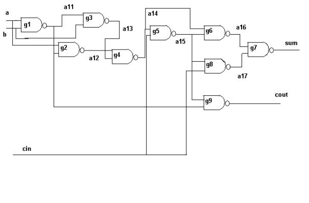
Fig.8.1. The simulated half-adder circuit.
To
completely calculate this example I had to change manually the input values and
calculate the result two times, once for the output ‘sum’ and once for the
output ‘cout’. This should be automated but in order to do so a few builtins
should be necessary.
The
circuit represents a halfadder. This is a typical example of a problem that certainly
can better be handled with forward reasoning. In backwards reasoning the
inferencing starts with gate g9 or
gate g7. All the possible input
values of these gates must be taken into consideration. In forward reasoning
the input values a and b immediately give the output of gate g1, g1 and a give the output
of gate g2 and so on…
The
source
Definition
of a half adder. The gate schema is taken from Wos[WOS].
definition
of a nand gate
The
definition of a nand gate consists of 4
rules. The nand gate is indicated by a variable G. The inputs are indicated by
the variables A and B. The output is indicated by the variable C. This is done
with the predicates gnand1, gnand2 and gnand3. A value is assigned to the
inputs using the predicates nand1 and nand2. The rule then inferes the value of
the output giving the predicate nand3.
gnand1(G,A),gnand2(G,B),gnand3(G,C),nand1(A,"false"),nand2(B,"false")
:> nand3(C,"true").
gnand1(G,A),gnand2(G,B),gnand3(G,C),nand1(A,"false"),nand2(B,"true")
:> nand3(C,"true").
gnand1(G,A),gnand2(G,B),gnand3(G,C),nand1(A,"true"),nand2(B,"false")
:> nand3(C,"true").
gnand1(G,A),gnand2(G,B),gnand3(G,C),nand1(A,"true"),nand2(B,"true")
:> nand3(C,"false").
definition
of the connection between gates
Two
rules define the connections between the different nand gates. There is a
nandnand2 connection when the output of a gate is connected with input 2 of the
following gate and there is a nandnand1 connection when the output is connected
with input 1.
nandnand2(G1,G2),gnand3(G1,X),gnand2(G2,X),nand3(X,V)
:> nand2(X,V).
nandnand1(G1,G2),gnand3(G1,X),gnand1(G2,X),nand3(X,V)
:> nand1(X,V).
An
example of a connection between two gates. I this case the output of gate 1 is
connected to both inputs of gate 2.
gnand1(g1,a).
gnand2(g1,b).
gnand3(g1,c).
nand1(a,"true").
nand2(b,"false").
nandnand1(g1,g2).
nandnand2(g1,g2).
gnand1(g2,c).
gnand2(g2,c).
gnand3(g2,d).
8.7. A description of owls.
This
case study shows that it is possible to put data into RDF format in a
systematic way. Queries can easily be done on this data. A GUI system could be
put on top for entering the data and for querying in a user friendly way.
A
query window can give e.g. lists of used URI’s.
8.8. A simulation of a flight reservation
I want to reserve a place in a flight going from
Zaventem (Brussels) to Rio de Janeiro. The flight starts on next Tuesday (for
simplicity only Tuesday is indicated as date).
Three servers are defined:
myServer
contains the files: flight_rules.pro and trust.pro.
airInfo
contains the file: air_info.pro.
intAir
contains the file: International_air.pro.
Namespaces are given by: http://thesis/inf , abbreviated inf, the engine system space
http://thesis:flight_rules,
abbreviated frul,the flight rules.
http://thesis/trust,
abbreviated trust, the trust
namespace.
http://flight_ontology/font,
abbreviated font, the flight ontology
space
http://international_air/air,
abbreviated air, the namespace of the
International Air company.
http://air_info/airinfo,
abbreviated ainf, the namespace of
the air information service.
These are non-existent namespaces created for the
purpose of this simulation..
The process goes as follows:
1)
start the query. The query contains an instruction for
loading the flight rules.
2)
Load the flight rules (module flight_rules.pro) in G2.
3)
Make the query for a flight Zaventem – Rio.
4)
The flight rules will direct a query to air info. This is done using the
predicate query.
5)
Air info answers: yes, the company is International
Air.
6)
The flight rules will consult the trust rules: module
trust.pro. This is done by directing a query to itself.
7)
The flight rules ask whether the company International
Air can be trusted.
8)
The trust module answers yes, so a query is directed
to International Air for commanding a ticket.
9)
International
Air answers with a confirmation of the reservation.
The reservation info is signalled to the user. The user is informed of the results (query + info + proof).
The content of the files can be found in annexe 3.
Chapter
9. Conclusion
9.1.Introduction
The goal of the Semantic Web
is to automate processes happening on the World Wide Web that are done manually
now. Seen the diversity of problems that can arise due to this goal, it is
clear that very general inferencing
engines will be needed. A basic engine is needed as a common platform that,
however, has a very modular structure such that it can be easily extended and
work together with other engines.
9.2.Characteristics of an inference engine
Taking into account the description of the goals of
the Semantic Web and examples thereof [TBL,TBL01,DEROO] it is possible and
necessary to deduce a list of characteristics that an inference engine for the
Semantic Web should have.
1)
Trust: the notion of trust has an important role in
the Semantic Web. If exchanges between computers have to be done in an automatic
way a computer on one site must be able to trust the computer at the other
side. To determine who can be trusted and who not a policy is necessary. When
the interchanges become fully automatic those policies will become complicated
sets of facts and rules. Therefore the necessity for an inference engine that
can make deductions from such a set. When deducing whether a certain source can
be trusted or not the property of monotonicity
is desirable: the decision on trustworthiness should not be changed after
loading e.g. another rule set.
2)
Inconsistencies and truth: if inconsistencies are
encountered e.g. site A says a person
is authenticated to do something and site B
says this person is not, the ‘truth’ is determined by the rules of trust: site A e.g. will be trusted and site B not. So truth does not have anymore an
absolute value.
1 & 2 imply that the engine should be coupled to the trust system. It
is the trust system that will give the possibility for verifying the ‘truth
value’ of a triple.
3)
Reasoning in a closed world often not is possible
anymore. A query ‘is x a mammal’ will
have no response at if x cannot be
found; the engine might find: x is a
bird but can this be trusted? Prolog would suppose that all mammals are known
in its database and when it does not find x
to be a mammal it would say: ‘x is not a
mammal’. However on the internet it is not possible to assume that ‘x is not a mammal’. The world is open
and in general sets should not be considered to be complete. This might pose
some problems with OWL and especially with that part of the ontology that
handles sets like intersection, complement of etc.. How to find the complement
of a set in an open world?
4)
An open world means also heterogenous information. The
engine can fetch or use facts and rules coming from anywhere. So finally it
might use a database composed with data and rules from different sites that
contains inconsistencies and contradictions. This poses the problem of the
detection of such inconsistencies. This again is also linked to the trust
system.
5)
In general
proving a theorem even in propositional calculus cannot be done in a fully
automatic way. [Wos]. As the Semantic Web talks about automatic interchange
this means that it should not be done. So the engine will be limited to querying
and proof verification.
6)
The existence of a Semantic Web means cooperation.
Cooperation means people and their machines following the rules: the standards.
The engine must work with the existing standards. There might be different
standards doing the same thing. This implies the existence of conversions e.g.
rule sets for the engine that convert between systems. This thesis considers
the standards XML, RDF, RDFS, OWL without therefore saying that other standards
ought not to be considered. This does not imply that I always agree with all
features of these standards but, generally, nobody will ever agree with all
features of a standard. Nevertheless the standards are a necessity. Therefore
the standards will be followed in this thesis. It seems however permitted to
propose alternatives. For the logic of an inference engine no standards are
available (or consider proposition logics and FOL as standards? ). Important
standardisations efforts have to be done to assure compatibility between
inference engines. Anyhow, the more
standards the less well the cooperation will work. Following the standard RDF
has a lot of consequences: unification involves unifying sets of triples;
functions are not available. The input and the output of the inference engine
have to be in RDF. Also the trace must be in RDF for providing the possibility
of proof verification.
7)
When exchanging messages between civilians, companies,
government and other parties the less point to point agreements have to be made
the more easy the process will become. This implies the existence of a standard
ontology (or ontologies). If agreement could be reached about some e.g. ±
1000 ontological concepts and their semantic effects on the level of a
computer, the interchange of messages between parties on the internet could
become a lot more easy. This implies that the internet inference engines will
have to work with ontologies. Possibly however this ontological material can be
translated to FOL terms.
8)
The engine has to be extensible in an easy way: an API
must exist that allows easy insertion of plugins. This API of course must be
standardised.
9)
The engine must have a model implementation that is
open source and has a structure that is easy to understand (as far as this is
possible) so that everybody can get acquainted in an easy way with the most
important principles.
10) All interchanges should be fully automatic (which is why the Semantic Web is made in the first place). Human interventions should only happen when the trust policies are unable to take a decision or their rules prescribe a human intervention.
11) The engine must be able to work with namespaces so that the origin of every notion can be traced.
12) As facts and rules are downloaded from different internet sites and loaded into the engine, the possibility must exist also to unload them. So it must be possible to separate again files that have been merged. The engine should also be able to direct queries to different rule sets.
13) The engine must be very fast as very large facts and rules bases can exist e.g. when the contents of a relational database are transformed to RDF. This thesis has a few suggestions for making a fast engine . On of them implicates making a typed resolution engine; the other is item 14.
14) Concurrency: this can happen on different levels: the search for alternatives can be done concurrently over different parts of the database; the validity of several alternatives can be checked concurrently; several queries can be done concurrently i.e. the engine can duplicated in different threads.
15) Duplicating the engine in several threads also means that it must be lightweight or reentrant.
16) There should be a minimal set of builtins representing functions that are commonly found in computer languages, theorem provers and query engines like: lists, mathemathical functions, strings, arrays and hashtables.
17) Existing theorem provers can be used using an API that permits a plugin to transform the standard database structure to the internal structure of the theorem prover. However, as detailed in the following texts, this is not an evident thing to do. As a matter of fact I argue that it is better to write new engines destined specifically for use in the Semantic Web.
18) FOL technologies are a possibility: resolution can be used; also Gentzen calculus or natural deduction could be used; CWM [SWAP] uses forward reasoning. This thesis will be based on a basic resolution engine. For more information on other logic techniques see a introductory handbook on logic e.g. [BENTHEM]. Other techniques such as graph based reasoning are also possible.
9.3. An evaluation of the RDFEngine
RDFEngine, the engine made for this thesis, is an experimental engine. It does not represent all of the characteristics mentionned above.
Fig.9.1. compares RDFEngine with the list of characteristics.
9.4. Forward versus backwards reasoning
As appears from the testcases and also from the literature e.g. [ALVES] sometimes backwards reasoning is the most efficient, sometimes forward reasoning is the most efficient. In some cases like the example in chapter 8 with the electronic gates, the difference is huge. As I argued before an inference engine for the Semantic Web must be capable of solving a very large gamma of different problems.
An engine could be made that is capable of two
mechanisms: forward reasoning and backwards reasoning. There are different possibilities:
1)
the mechanism used is determined by an instruction in
the axiom file
2)
first one is used; if no positive result the other is
used
3)
both are used with a timeout
4)
both are used concurrently
I believe a basic engine for the semantic web
should be capable of using these two mechanisms. The Swich software uses a
graph matching algorithm that could be the basis for a third, general
inferencing mechanism, as was already mentionned in chapter 4.
9.5. Final conclusions
The
Semantic Web is a vast, new and highly experimental domain of research. This
thesis concentrates on a particular aspect of this reasearch domain i.e. RDF
and inferencing. In the layer model of the Semantic Web given in fig. 2.2 this
concerns the logic, proof and trust layers with the accent on the logic layer.
In chapter 1 the goals of the thesis were
exposed. I recapitulate them briefly:
1) What elements should be present in an inferencing standard for the Semantic Web?
2)
What system of logic is best suited for the Semantic
Web?
3)
What techniques can be used for optimization of the
engine?
4)
How must inconsistencies be handled?
1) A
trust system is not implemented. Nevertheless the modularity of the implemented
system permits to make a module containing trust rules. Operational aspects of
trust and cryptography can be added by adding builtins to the engine. The
property of monotonicity is respected by the engine.
2) All
statements are marked by provenance information. Whenever an inconsistency
arises it is possible to reject information having a certain origin. This can
be done by using rules and unloading the statements having a certain origin.
3) The
logic of RDFEngine is completely compatible with an open world as it has been
shown in chapter 3 and 5.
4) RDFEngine
can use information from different sites in a modular way.
5) RDFEngine can do
querying and proof verification; it is not impossible do to theorem proving
with it, though this is not the intention and probably will not be easy to do.
6) RDFEngine follows
the standards XML, RDF, RDFS.
Experiments have been done with certain OWL constructions.
7) OWL is not
implemented; however it is certainly possible using the defined structures.
8) An API for RDFEngine that intercepts the matching of
a clause and handles builtins or applies other inferencing to statements can
easily be made.
9) RDFEngine is open
source. Its workings are explained in chapter 3.
10) RDFEngine does not
need human intervention; it can however be programmed.
11) RDFEngine is apt to
work with namespaces.
12) RDFEngine can load
and unload modules. It can also work with virtuals servers. It can direct
queries to other servers and interprete the results.
13) The engine works
with a hashtable. This permits rapid retrieval of the relevant predicates for
unification. The highly modular structure also permits to limit the size of the
modules.
14) Concurrency is not
implemented.
15) Virtual servers can
easily be run in parallel via a socket system.
16) RDFEngine implements
some builtins. Adding other builtins is very easy.
17) Nothing to remark.
18) The structure of
RDFEngine is such that a combination of inferencing methods is possible.
Different virtual servers could use different inferencing mechanisms. They
communicate with each other using a standard interchange format for the
results. An experiment has not been done due to a lack of time.
The accent has been on points 1 and 2. This is largely
due to the fact that I encountered substantial theoretical problems when trying
to find an answer for these questions. Certainly, in view of the fact that the
Semantic Web must be fully automated, very clear definitions of the semantics
are needed in terms of computer operations.
The investigations into logic lead to the belief that
the fact that the World Wide Web is an open world is of the utmost importance.
This fact has a lot of logical consequences. Unevitably, the logic of the
internet must be seen in a constructive way i.e. something is only true if it
can be constructed. Constructive proofs also permit the verification of the
proof.
Generally, RDF inferencing can be approached from two angles. One
approach is based on First Order Logic(FOL). FOL is, of course, a very powerful
modelling tool. Nevertheless, bacause RDF is defined as a graph model, the
question arises whether this modelling using FOL is correct. In fact, all the constructive aspects of RDF
are lost in a FOL model. Constructive
logic is not First Order Logic.
On the other hand , a model of RDF and inferencing
based purely on a graph theoretical reasoning leads to very clear definitions
of rules, queries and solutions as was shown in chapter 3. With these
definitions is also possible to define an interchange format between reasoning
engines whathever the used reasoning method.
After numerous experiments a model of distributed
inferencing was developed.
The notion of inference step is defined. An inference
step is defined at the level of the unification of a statement (clause) with the
RDF graph. An inference step can redirect the inferencing process to a
different server. The inferencing process is under control of a main server who
uses secondary servers. Sub-queries are directed to the secondary servers. The
secondary servers return the results of the sub-query in a standard format. A
secondary server can use other inference mechanisms than the primary server.
The primary server will have the ability to acquire information about the
processes used on the secondary server like authorithy information, the used
inferencing processes etc…
The goal is to arrive at a cooperation of inferencing
mechanisms on the scale of the World Wide Web.
An extensive example of such a cooperative query is
provided.
Each server can make use of different RDF graphs. As
servers can be virtual this creates a double modular structure: low level
modules are constituted by RDF graphs and high level modules are constituted by
virtual servers who communicate between them using sockets. Different virtual
servers can use different inference mechanisms.
In chapter 5 a further reseach into the logic
properties of RDF and the proposed inferencing model is done with the renewed
conclusion that a kind of constructive logic is what is needed for the Semantic
Web.
An executable engine has been built in Haskell. The
characteristics of Haskell force the programmer to execute a separation of
concerns. The higher order functions permit to write very compact code. The
following programming model was used:
1)
define an abstract syntax corresponding to different
concrete syntaxes like RDFProlog and Notation 3.
2)
Encapsulate the data structures into an Abstract Data
Type (ADT).
3)
Define an interface language for the ADT’s, also
called mini-languages.
4)
Program the main functional parts of the program using
these mini-languages.
This programming model leads to very portable,
maintainable and data independent program structures.
Suggestions can be made for further research:
·
RDFEngine can be used as a simulation tool for
investigating the characteristics of distributed inferencing for several
different vertical application models. Examples are: placing a command, making
an appointment with a dentist, searching a book, etc…
·
The integration with trust systems and
cryptographic methods needs further study.
·
An interesting possibility is the build of inference engines that use both forward en
backwards reasoning or a mix of both.
·
Complementary to the previous point, the
feasability of an inference engine based on subgraph matching technologies
using the algorithm of Carroll is worth investigating.
·
The applicability of methods for enhancing the
efficiency of forwards reasoning in an RDF engine should be studied. It is
especially worth studying whether RDF permits special optimization techniques.
·
This is the same as previous item but for
backwards reasoning.
·
The interaction between different inference
engines can be further studied.
·
OWL (Lite) can be implemented and the
modalities of different implementations and ways of implementation can be
studied.
·
Which user interfaces are needed? What about
messages to the user?
·
A study can be made what meta information is
interesting to provide concerning the inference clients, engines, servers and
other entities.
·
A very interesting and, in my opinion, necessary
field of research is how Semantic Web engines will have learning capabilities.
A main motivation for this is the avoidance of repetitive queries with the same
result. Possibly also, clients can learn from the human user in case of
conflict.
·
Adding to the previous point, the study of
conflict resolving mechanisms is interesting. Inspiration can be sought with
the SOAR project.
·
Further study is necessary concerning
inferencing contexts. The Ph.D. thesis of Guha [GUHA] can serve as a starting
point.
·
How can proofs be transformed to procedures and
this in relation to learning as wel as optimization?
·
Implement a learning by example system as
indicated in chapter 6.
·
The definition of a tri-valued constructive
logic (true, false, don’t know).
I believe RDFEngine can be a starting point for
a ‘reference’ implementation of a
Semantic Web engine. It can also be a starting point for further
investigations. I hope that this thesis has given a small but significant contribution
to the development of the Semantic Web.
Bibliography
[AIT] Hassan Aït-Kaci WAM A tutorial reconstruction .
[ADDRESSING] http://www.w3.org/Adressing/ .
[ALBANY] http://www.albany.edu/~gilmr/metadata/rdf.ppt
[ALVES] Alves, Datalog,programmation logique et négation,Université de tours.
[BERNERS] Semantic Web Tutorial Using N3,Berners-Lee e.a., May 20,2003, http://www.w3.org/2000/10/swap/doc/
[BOLLEN] Bollen e.a., The World-Wide Web as a Super-Brain: from metaphor to model, http://pespmc1.vub.ac.be/papers/WWWSuperBRAIN.html
[BOTHNER] Per Bothner, What is Xquery?, http://www.xml.com/lpt/a/2002/10/16/xquery.html
[BUNDY] Alan
Bundy , Artificial Mathematicians,
May 23, 1996, http://www.dai.ed.ac.uk/homes/bundy/tmp/new-scientist.ps.gz
[CARROLL]
Carroll,J., Matching RDF Graphs, July 2001.
[CASTELLO] R.Castello e.a. Theorem provers survey. University of Texas at Dallas. http://citeseer.nj.nec.com/409959.html
[CENG] André Schoorl, Ceng 420 Artificial intelligence University of Victoria, http://www.engr.uvic.ca/~aschoorl/ceng420/
[CHAMPIN] Pierre Antoine Champin, 2001 – 04 –05, http://www710.univ-lyon1.fr/~champin/rdf-tutorial/node12.html
[CLUB]
http://www.cirl.uoregon.edu/~iustin/cis571/unit3.html,
University of Oregon
[COQ] Huet e.a. RT-0204-The Coq Proof Assistant : A Tutorial, http://www.inria.fr/rrt/rt-0204.html.
[CS] http://www.cs.ucc.ie/~dgb/courses/pil/ws11.ps.gz
[DAML+OIL] DAML+OIL (March 2001)
Reference Description. Dan Connolly, Frank
van Harmelen, Ian Horrocks, Deborah L. McGuinness, Peter F. Patel-Schneider,
and Lynn Andrea Stein. W3C Note 18 December 2001. Latest version is available
at http://www.w3.org/TR/daml+oil-reference.
[DECKER] Decker e.a., A query and Inference Service for RDF,University of KarlsRuhe.
[DENNIS] Louise Dennis Midlands Graduate School in TCS, http://www.cs.nott.ac.uk/~lad/MR/lcf-handout.pdf
[DESIGN] http://www.w3.org/DesignIssues/
* Tim Berners-Lee’s site with his
design-issues articles .
[DEROO]
http://www.agfa.com/w3c/jdroo * the site of the Euler program
[DICK] A.J.J.Dick, Automated equational
reasoning and the knuth-bendix algorithm: an informal introduction, Rutherford
Appleton Laboratory Chilton, Didcot OXON OX11 OQ,
http://www.site.uottawa.ca/~luigi/csi5109/church-rosser.doc/
[DONALD] http://dream.dai.ed.ac.uk/papers/donald/subsectionstar4_7.html
[EDMONDS] Edmonds Bruce, What if all truth is context-dependent?, Manchester Metropolitan
University, http://www.cpm.mmu.ac.uk/~bruce.
[GANDALF]
http://www.cs.chalmers.se/~tammet/gandalf * Gandalf Home Page
[GENESERETH] Michael Genesereth, Course Computational logic, Computer Science Department, Stanford University.
[GHEZZI] Ghezzi e.a. Fundamentals of Software Engineering Prentice-Hall 1991 .
[GRAPH] http://www.agfa.com/w3c/euler/graph.axiom.n3
[GROSOF]Benjamin
Grosof, Introduction to RuleML, http://ebusiness.mit.edu/bgrosof/paps/talk-ruleml-jc-ovw-102902-main.pdf
[GUHA] R. V. Guha, Contexts: A formalization and some applications,
MCC Technical Report No. ACT-CYC-423-91, November 1991.
[GUPTA] Amit Gupta & Ashutosh Agte, Untyped lambda calculus, alpha-, beta- and
eta- reductions, April 28/May 1 2000, http://www/cis/ksu.edu/~stefan/Teaching/CIS705/Reports/GuptaAgte-2.pdf
[HARRISON] J.Harrison, Introduction to functional programming, 1997.
[HAWKE] http://lists.w3.org/Archives/Public/www-rdf-rules/2001Sep/0029.html
[HEFLIN] J.D.Heflin, Towards the semantic web: knowledge representation in a dynamic,distributed environment, Dissertation 2001.
[HILOG] http://www.cs.sunysb.edu/~warren/xsbbook/node45.html
[JEURING]
J.Jeuring and D.Swierstra, Grammars and
parsing, http://www.cs.uu.nl/docs/vakken/gont/
[JEURING1]
Jeuring e.a. ,Polytypic unification, J.Functional
programming, september 1998.
[KERBER] Manfred Kerber, Mechanised Reasoning, Midlands Graduate School in Theoretical
Computer Science, The University of Birmingham, November/December 1999, http://www.cs.bham.ac.uk/~mmk/courses/MGS/index.html
[KLYNE]G.Klyne, Nine by nine:Semantic Web Inference using Haskell, May, 2003, http://www/ninebynine.org/Software/swish-0.1.html
[KLYNE2002] G.Klyne,Circumstance, provenance and partial knowledge,
http://www.ninebyne.org/RDFNotes/UsingContextsWithRDF.html
[LAMBDA] http://www.cse.psu.edu/~dale/lProlog/ * lambda
prolog home page
[LEHMAN] Lehman e.a., A gentle Introduction to Soar, an Architecture for Human Cognition.
[LINDHOLM] Lindholm, Exercise Assignment Theorem prover for propositional modal logics, http://www.cs.hut.fi/~ctl/promod.ps
[LOGPRINC] http://www.earlham.edu/~peters/courses/logsys/glossary.html
[MCGUINESS] Deborah McGuiness Explaining reasoning in description logics 1966 Ph.D.Thesis
[MCGUINESS2003] McGuiness e.a., Inference Web:Portable explanations for the
web,Knowledge Systems Laboratory, Stanford University.
[MYERS] CS611 LECTURE 14 The Curry-Howard Isomorphism, Andrew Myers.
[NADA] Arthur Ehrencrona, Royal Institute of Technology Stockholm, Sweden, http://cgi.student.nada.kth.se/cgi-bin/d95-aeh/get/umeng
[NUPRL] http://www.nuprl.org/Intro/Logic/logic.html
[OTTER] http://www.mcs.anl.gov/AR/otter/ Otter
Home Page
[OWL Features] Feature Synopsis for OWL Lite and OWL. Deborah L. McGuinness and Frank van Harmelen. W3C Working Draft 29 July
2002. Latest version is available at http://www.w3.org/TR/owl-features/.
[OWL Issues] Web Ontology Issue Status. Michael K. Smith, ed. 10 Jul 2002.
[OWL Reference] OWL Web
Ontology Language 1.0 Reference. Mike Dean, Dan
Connolly, Frank van Harmelen, James Hendler, Ian Horrocks, Deborah L.
McGuinness, Peter F. Patel-Schneider, and Lynn Andrea Stein. W3C Working Draft
29 July 2002. Latest version is available at http://www.w3.org/TR/owl-ref/.
[OWL Rules] http://www.agfa.com/w3c/euler/owl-rules
[PFENNING_1999] Pfenning e.a., Twelf a Meta-Logical framework for deductive Systems, Department of Computer Science, Carnegie Mellon University, 1999.
[PFENNING_LF] http://www-2.cs.cmu.edu/afs/cs/user/fp/www/lfs.html
[POPPER]Bryan Magee, Popper, Het
Spectrum, 1974.
[RDFM]RDF
Model Theory .Editor: Patrick Hayes
http://www.w3.org/TR/rdf-mt/
[RDFMS] Resource
Description Framework (RDF) Model and Syntax Specification http://www.w3.org/TR/1999/REC-rdf-syntax-19990222
[RDFPRIMER] http://www.w3.org/TR/rdf-primer/
[RDFRULES]
http://lists.w3.org/Archives/Public/www-rdf-rules/
[RDFSC] Resource
Description Framework (RDF) Schema Specification 1.0 http://www.w3.org/TR/2000/CR-rdf-schema-20000327
[RQL] Sesame RQL :a Tutorial,J.Broekstra,
http://sesame.aidministrator.nl/publications/rql-tutorial.html
[SABIN]
Miles Sabin, http://lists.w3.org/Archives/Public/www-rdf-logic/2001Apr/0074.html
[SCHNEIER]
Schneier Bruce, Applied Cryptography
[SINTEK] Sintek e.a.,TRIPLE – A query, Inference, and
Transformation Language for the Semantic Web, Stanford University.)
[STANFORD] Portoraro, Frederic, "Automated Reasoning", The Stanford Encyclopedia of Philosophy (Fall 2001 Edition), Edward N. Zalta (ed.), http://plato.stanford.edu/archives/fall2001/entries/reasoning-automated/.
[STANFORDP] Priest, Graham, Tanaka, Koji,
"Paraconsistent Logic", The Stanford Encyclopedia of Philosophy
(Winter 2000 Edition), Edward N. Zalta (ed.), http://plato.stanford.edu/archives/win2000/entries/logic-paraconsistent/.
[SWAP/CWM] http://www.w3.org/2000/10/swap http://infomesh.net/2001/cwm CWM is another inference engine for
the web .
[SWAPLOG] http://www/w3.org/200/10/swap/log#
[TBL] Tim-berners Lee, Weaving the web,
[TBL01] Berners-Lee e.a.The semantic web Scientific American May 2001
[TWELF] http://www.cs.cmu.edu/~twelf*
Twelf Home Page
[UNCERT] Hin-Kwong Ng e.a. Modelling uncertainties in argumentation, Department of Systems Engineering &
Engineering Management The Chinese University of Hong Kong http://www.se.cuhk.edu.hk/~hkng/papers/uai98/uai98.html
[UNICODE] http://www.unicode.org/unicode/standard/principles.html
[UMBC] TimothyW.Finin, Computer Science and Electrical Engineering, University of Maryland Baltimore Country, http://www.cs.umbc.edu/471/lectures/9/sld040.htm
[URI] http://www.isi.edu/in-notes/rfc2396.txt
[USHOLD] Michael Ushold The boeing company, Where is the semantics of the web?http://cis.otago.ac.nz/OASWorkschop/Papers/WhereIsTheSemantics.pdf
[VAN BENTHEM] Van Benthem e.a.,
Logica voor informatici, Addison Wesley 1991.
[WALSH] Toby Walsh, A divergence critic for inductive proof, 1/96, Journal of
Artificial Intelligence Research, http://www-2.cs.cmu.edu/afs/cs/project/jair/pub/volume4/walsh96a-html/section3_3.html
[WESTER] Wester e.a. Concepten van programmeertalen,Open Universiteit Eerste druk 1994 Important for a thorough introduction in Gofer
. In Dutch .
[WOS] Wos e.a. Automated reasoning,Prentice Hall, 1984
[W3SCHOOLS http://www.w3schools.com/w3c/w3c_intro.asp
[YUREK] Yurek , Datalog
bottom-up is the trend in the deductive database evaluation strategy,
University of Maryland, 2002.
List of abbreviations
ALF : Algebraic Logic Functional Programming
Language
API : Application Programming Interface
CA : Certification Authority
CWM : Closed World Machine
An experimental inference engine for the
semantic web
DTD : Document Type Definition , a language for
defining XML-
objects .
HTML : Hypertext Markup Language
KB : Knowledge Base
FOL : First Order Logic
N3 : Notation 3
OWL : Ontology Web Language
PKI : Public Key Infrastructure
RA : Registration Authority
RDF : Resource Description Framework
RDFS : RDF Schema
SGML : Standard General Markup Language
SweLL : Semantic Web Logic Language
URI : Uniform Resource Indicator
URL : Uniform Resource Locator
W3C : World Wide Web Consortium
WAM : Warren Abstract Machine
Probably the first efficient implementation
of prolog .
XML : Extensible Markup Language .
The difference with HTML is that tags can be
freely defined in
XML .
Appendix 1: Excuting the
engine
There are
actually two versions of the engine. One, N3Engine has been tested with a lot
of usecases buthas a rather conventional structure. The other, RDFEngine, is
less tested but has a structure that is more directed towards the Semantic Web.
It is the version RDFEngine that has been exposed in the text and of which the
source code is added at the end.
Usage of the inference engine N3Engine.
First unzip the file EngZip.zip into a directory.
Following steps construct a demo (with the Hugs distribution under Windows):
1) winhugs.exe
2) :l RDFProlog.hs
3) menu
4) choose one of the examples e.g. en2. These are testcases with the source
in Notation 3
5) menuR
6) choose one of the examples e.g. pr12. Those with number 1 at the end
give the translation from RDFProlog to Notation3; those with number 2 at the
end execute the program.
Usage of the inference engine RDFEngine.
First unzip the file RDFZip.zip into a directory.
Following steps construct a demo (with the Hugs distribution under Windows):
7) winhugs.exe
8) :l RDFEngine.hs
9) pro11
10)repeat the s(tep) instruction
or after
loading:
9) start
10) menu
11) choose an item
12) enter e
Appendix 2. Example of a closure path.
An
example of a resolution and a closure path made with the gedcom example (files
gedcom.facts.n3, gedcom.relations.n3, gedcom.query.n3)
First the trace is given with the global
substitutions and all calls and alternatives:
Substitutions:
{2$_$17_:child = :Frank. _1?who1 =
2$_$17_:grandparent. 3$_$16_:child = :Frank. 2$_$17_:grandparent =
3$_$16_:grandparent. 4$_$13_:child = :Frank. 3$_$16_:parent = 4$_$13_:parent.
4$_$13_:family = :Naudts_VanNoten. 4$_$13_:parent = :Guido. 7$_$13_:child =
:Guido. 3$_$16_:grandparent = 7$_$13_:parent. 7$_$13_:family =
:Naudts_Huybrechs. 7$_$13_:parent = :Pol. }.
N3Trace:
[:call {:Frank gc:grandfather _1?who1. }].
:alternatives = {{2$_$17_:child gc:grandparent
2$_$17_:grandparent. 2$_$17_:grandparent gc:sex :M. }
}
[:call {:Frank gc:grandparent
2$_$17_:grandparent. }].
:alternatives = {{3$_$16_:child gc:parent
3$_$16_:parent. 3$_$16_:parent gc:parent 3$_$16_:grandparent. }
}
[:call {:Frank gc:parent 3$_$16_:parent. }].
:alternatives = {{4$_$13_:child gc:childIn
4$_$13_:family. 4$_$13_:parent gc:spouseIn 4$_$13_:family. }
}
[:call {:Frank gc:childIn 4$_$13_:family. }].
:alternatives = {{:Frank gc:childIn
:Naudts_VanNoten. }
}
[:call {4$_$13_:parent gc:spouseIn
:Naudts_VanNoten. }].
:alternatives = {{:Guido gc:spouseIn
:Naudts_VanNoten. }
{:Christine gc:spouseIn :Naudts_VanNoten. }
}
[:call {:Guido gc:parent 3$_$16_:grandparent.
}].
:alternatives = {{7$_$13_:child gc:childIn
7$_$13_:family. 7$_$13_:parent gc:spouseIn 7$_$13_:family. }
}
[:call {:Guido gc:childIn 7$_$13_:family. }].
:alternatives = {{:Guido gc:childIn
:Naudts_Huybrechs. }
}
[:call {7$_$13_:parent gc:spouseIn
:Naudts_Huybrechs. }].
:alternatives = {{:Martha gc:spouseIn
:Naudts_Huybrechs. }
{:Pol gc:spouseIn :Naudts_Huybrechs. }
}
[:call {:Pol gc:sex :M. }].
:alternatives = {{:Pol gc:sex :M. }
}
Query:
{:Frank gc:grandfather _1?who1. }
Solution:
{:Frank gc:grandfather :Pol. }
The calls and alternatives with the global
substitution applied:
------------------------------------------------------------------
It can be immediately verified that the
resolution path is complete.
(The alternatives that lead to failure are
deleted).
[:call {:Frank gc:grandfather :Pol.}].
:alternatives = {{:Frank gc:grandparent :Pol.
:Pol gc:sex :M. }
}
[:call {:Frank gc:grandparent :Pol. }].
:alternatives = {{:Frank gc:parent :Guido.
:Guido gc:parent :Pol. }
}
[:call {:Frank gc:parent :Guido. }].
:alternatives = {{:Frank gc:childIn
:Naudts_Vannoten. :Guido gc:spouseIn :Naudts_Vannoten. }
}
[:call {:Frank gc:childIn :Naudts_Vannoten. }].
:alternatives = {{:Frank gc:childIn
:Naudts_VanNoten. }
}
[:call {:Guido gc:spouseIn :Naudts_VanNoten.
}].
:alternatives = {{:Guido gc:spouseIn
:Naudts_VanNoten. }
}
[:call {:Guido gc:parent :Pol. }].
:alternatives = {{:Guido gc:childIn
:Naudts_Huybrechs. :Pol gc:spouseIn :Naudts_Huybrechs. }
}
[:call {:Guido gc:childIn :Naudts_Huybrechs.
}].
:alternatives = {{:Guido gc:childIn
:Naudts_Huybrechs. }
}
[:call {:Pol gc:spouseIn :Naudts_Huybrechs. }].
:alternatives = {{:Pol gc:spouseIn
:Naudts_Huybrechs. }
}
[:call {:Pol gc:sex :M. }].
:alternatives = {{:Pol gc:sex :M. }
}
Query:
{:Frank gc:grandfather _1?who1. }
Solution:
{:Frank gc:grandfather :Pol. }
It is now possible to establish the closure
path.
( {{:Guido gc:childIn :Naudts_Huybrechs. :Pol
gc:spouseIn :Naudts_Huybrechs. }, {:Guido gc:parent :Pol. })
( {{:Frank gc:childIn :Naudts_Vannoten. :Guido
gc:spouseIn :Naudts_Vannoten. }, {:Frank gc:parent :Guido. })
({{:Frank gc:parent :Guido. :Guido gc:parent
:Pol. },
{:Frank gc:grandparent :Pol. })
({{:Frank gc:grandparent :Pol. :Pol gc:sex :M.
},
{:Frank gc:grandfather :Pol.})
The triples that were added during the closure
are:
{:Guido gc:parent :Pol. }
{:Frank gc:parent :Guido. }
{:Frank gc:grandparent :Pol. }
{:Frank gc:grandfather :Pol.}
It is verified that the reverse of the
resolution path is indeed a closure path.
Verification of the lemmas
----------------------------
Closure Lemma: certainly valid for this closure
path.
Query Lemma: the last triple in the closure
path is the query.
Final Path Lemma: correct for this resolution
path.
Looping Lemma: not applicable
Duplication Lemma: not applicable.
Failure Lemma: not contradicted.
Solution Lemma I: correct for this testcase.
Solution Lemma II: correct for this testcase.
Solution Lemma III: not contradicted.
Completeness Lemma: not contradicted.
Appendix 3. Test cases
Gedcom
The file
with the relations (rules):
# $Id: gedcom-relations.n3,v 1.3 2001/11/26 08:42:34 amdus Exp $
# Original http://www.daml.org/2001/01/gedcom/gedcom-relations.xml by Mike Dean (BBN Technologies / Verizon)
# Rewritten in N3 (Jos De Roo AGFA)
# state that the rules are true (made by Tim Berners-Lee W3C)
# see also http://www.w3.org/2000/10/swap/Examples.html
@prefix log:
<http://www.w3.org/2000/10/swap/log#> .
@prefix ont:
<http://www.daml.org/2001/03/daml+oil#> .
@prefix gc: <http://www.daml.org/2001/01/gedcom/gedcom#> .
@prefix : <gedcom#> .
{{:child gc:childIn :family. :parent gc:spouseIn :family} log:implies {:child gc:parent :parent}} a log:Truth; log:forAll :child, :family, :parent.
{{:child gc:parent :parent. :parent gc:sex :M} log:implies {:child gc:father :parent}} a log:Truth; log:forAll :child, :parent.
{{:child gc:parent :parent. :parent gc:sex :F} log:implies {:child gc:mother :parent}} a log:Truth; log:forAll :child, :parent.
{{:child gc:parent :parent} log:implies {:parent gc:child :child}} a log:Truth; log:forAll :child, :parent.
{{:child gc:parent :parent. :child gc:sex :M} log:implies {:parent gc:son :child}} a log:Truth; log:forAll :child, :parent.
{{:child gc:parent :parent. :child gc:sex :F} log:implies {:parent gc:daughter :child}} a log:Truth; log:forAll :child, :parent.
{{:child gc:parent :parent. :parent gc:parent :grandparent} log:implies {:child gc:grandparent :grandparent}} a log:Truth; log:forAll :child, :parent, :grandparent.
{{:child gc:grandparent :grandparent. :grandparent gc:sex :M} log:implies {:child gc:grandfather :grandparent}} a log:Truth; log:forAll :child, :parent, :grandparent.
{{:child gc:grandparent :grandparent. :grandparent gc:sex :F} log:implies {:child gc:grandmother :grandparent}} a log:Truth; log:forAll :child, :parent, :grandparent.
{{:child gc:grandparent :grandparent} log:implies {:grandparent gc:grandchild :child}} a log:Truth; log:forAll :child, :grandparent.
{{:child gc:grandparent :grandparent. :child gc:sex :M} log:implies {:grandparent gc:grandson :child}} a log:Truth; log:forAll :child, :grandparent.
{{:child gc:grandparent :grandparent. :child gc:sex :F} log:implies {:grandparent gc:granddaughter :child}} a log:Truth; log:forAll :child, :grandparent.
{{:child1 gc:childIn :family. :child2 gc:childIn :family. :child1 ont:differentIndividualFrom :child2} log:implies {:child1 gc:sibling :child2}} a log:Truth; log:forAll :child1, :child2, :family.
{{:child2 gc:sibling :child1} log:implies {:child1 gc:sibling :child2}} a log:Truth; log:forAll :child1, :child2.
{{:child gc:sibling :sibling. :sibling gc:sex :M} log:implies {:child gc:brother :sibling}} a log:Truth; log:forAll :child, :sibling.
{{:child gc:sibling :sibling. :sibling gc:sex :F} log:implies {:child gc:sister :sibling}} a log:Truth; log:forAll :child, :sibling.
{?a gc:sex :F. ?b gc:sex :M.} log:implies {?a ont:differentIndividualFrom ?b.}.
{?b gc:sex :F. ?a gc:sex :M.} log:implies {?a ont:differentIndividualFrom ?b.}.
{{:spouse1 gc:spouseIn :family. :spouse2 gc:spouseIn :family. :spouse1 ont:differentIndividualFrom :spouse2} log:implies {:spouse1 gc:spouse :spouse2}} a log:Truth; log:forAll :spouse1, :spouse2, :family.
{{:spouse2 gc:spouse :spouse1} log:implies {:spouse1 gc:spouse :spouse2}} a log:Truth; log:forAll :spouse1, :spouse2.
{{:spouse gc:spouse :husband. :husband gc:sex :M} log:implies {:spouse gc:husband :husband}} a log:Truth; log:forAll :spouse, :husband.
{{:spouse gc:spouse :wife. :wife gc:sex :F} log:implies {:spouse gc:wife :wife}} a log:Truth; log:forAll :spouse, :wife.
{{:child gc:parent :parent. :parent gc:brother :uncle} log:implies {:child gc:uncle :uncle}} a log:Truth; log:forAll :child, :uncle, :parent.
{{:child gc:aunt :aunt. :aunt gc:spouse :uncle} log:implies {:child gc:uncle :uncle}} a log:Truth; log:forAll :child, :uncle, :aunt.
{{:child gc:parent :parent. :parent gc:sister :aunt} log:implies {:child gc:aunt :aunt}} a log:Truth; log:forAll :child, :aunt, :parent.
{{:child gc:uncle :uncle. :uncle gc:spouse :aunt} log:implies {:child gc:aunt :aunt}} a log:Truth; log:forAll :child, :uncle, :aunt.
{{:parent gc:daughter :child. :parent gc:sibling :sibling} log:implies {:sibling gc:niece :child}} a log:Truth; log:forAll :sibling, :child, :parent.
{{:parent gc:son :child. :parent gc:sibling :sibling} log:implies {:sibling gc:nephew :child}} a log:Truth; log:forAll :sibling, :child, :parent.
{{:cousin1 gc:parent :sibling1. :cousin2 gc:parent :sibling2. :sibling1 gc:sibling :sibling2} log:implies {:cousin1 gc:firstCousin :cousin2}} a log:Truth; log:forAll :cousin1, :cousin2, :sibling1, :sibling2.
{{:child gc:parent :parent} log:implies {:child gc:ancestor :parent}} a log:Truth; log:forAll :child, :parent.
{{:child gc:parent :parent. :parent gc:ancestor :ancestor} log:implies {:child gc:ancestor :ancestor}} a log:Truth; log:forAll :child, :parent, :ancestor.
{{:child gc:ancestor :ancestor} log:implies {:ancestor gc:descendent :child}} a log:Truth; log:forAll :child, :ancestor.
{{:sibling1 gc:sibling :sibling2. :sibling1 gc:descendent :descendent1. :sibling2 gc:descendent :descendent2} log:implies {:descendent1 gc:cousin :descendent2}} a log:Truth; log:forAll :descendent1, :descendent2, :sibling1, :sibling2.
The file with the facts:
# $Id: gedcom-facts.n3,v 1.3 2001/11/26 08:42:33 amdus Exp $
@prefix gc: <http://www.daml.org/2001/01/gedcom/gedcom#>.
@prefix log: <http://www.w3.org/2000/10/swap/log#>.
@prefix : <gedcom#>.
:Goedele gc:childIn :dt; gc:sex :F.
:Veerle gc:childIn :dt; gc:sex :F.
:Nele gc:childIn :dt; gc:sex :F.
:Karel gc:childIn :dt; gc:sex :M.
:Maaike gc:spouseIn :dt; gc:sex :F.
:Jos gc:spouseIn :dt; gc:sex :M.
:Jos gc:childIn :dp; gc:sex :M.
:Rita gc:childIn :dp; gc:sex :F.
:Geert gc:childIn :dp; gc:sex :M.
:Caroline gc:childIn :dp; gc:sex :F.
:Dirk gc:childIn :dp; gc:sex :M.
:Greta gc:childIn :dp; gc:sex :F.
:Maria gc:spouseIn :dp; gc:sex :F.
:Frans gc:spouseIn :dp; gc:sex :M.
:Ann gc:childIn :gd; gc:sex :F.
:Bart gc:childIn :gd; gc:sex :M.
:Rita gc:spouseIn :gd; gc:sex :F.
:Paul gc:spouseIn :gd; gc:sex :M.
:Ann_Sophie gc:childIn :dv; gc:sex :F.
:Valerie gc:childIn :dv; gc:sex :F.
:Stephanie gc:childIn :dv; gc:sex :F.
:Louise gc:childIn :dv; gc:sex :F.
:Christine gc:spouseIn :dv; gc:sex :F.
:Geert gc:spouseIn :dv; gc:sex :M.
:Bieke gc:childIn :cd; gc:sex :F.
:Tineke gc:childIn :cd; gc:sex :F.
:Caroline gc:spouseIn :cd; gc:sex :F.
:Hendrik gc:spouseIn :cd; gc:sex :M.
:Frederik gc:childIn :dc; gc:sex :M.
:Stefanie gc:childIn :dc; gc:sex :F.
:Stijn gc:childIn :dc; gc:sex :M.
:Karolien gc:spouseIn :dc; gc:sex :F.
:Dirk gc:spouseIn :dc; gc:sex :M.
:Lien gc:childIn :sd; gc:sex :F.
:Tom gc:childIn :sd; gc:sex :M.
:Greta gc:spouseIn :sd; gc:sex :F.
:Marc gc:spouseIn :sd; gc:sex :M.
The queries:
# $Id: gedcom-query.n3,v 1.5 2001/12/01 01:21:27 amdus Exp $
# PxButton | test | jview Euler gedcom-relations.n3 gedcom-facts.n3 gedcom-query.n3 |
@prefix log:
<http://www.w3.org/2000/10/swap/log#>.
@prefix gc: <http://www.daml.org/2001/01/gedcom/gedcom#>.
@prefix : <gedcom#>.
# _:x gc:parent :Maaike, :Jos. # ok
# :Maaike gc:son _:x. # ok
# :Jos gc:daughter _:x. # ok
# _:x gc:grandfather :Frans. # ok
# :Maria gc:grandson _:x. # ok
:Frans gc:granddaughter _:x. # ok
# :Nele gc:sibling _:x. # ok
# _:x gc:brother :Geert. # ok
# _:x gc:spouse :Frans. # ok
# _:x gc:husband _:y. # ok
# :Karel gc:aunt _:x. # ok
# :Nele gc:aunt _:x. # ok
# :Rita gc:niece _:x.
# :Nele gc:firstCousin _:x.
# :Karel
gc:ancestor _:x. # ok
# :Maria gc:descendent _:x. # ok
# :Karel gc:cousin _:x. # ok
Ontology
The axiom
file:
#
File ontology1.axiom.n3
#
definition of rdfs ontology
#
modelled after: A Logical Interpretation of RDF
#
Wolfram Conen, Reinhold Klapsing, XONAR IT and Information Systems
# and
Software Techniques Velbert, Germany U Essen, D-45117
@prefix
log: <http://www.w3.org/2000/10/swap/log#>.
@prefix
ont: <http://www.w3.org/2002/07/daml+oil#> .
@prefix
owl: <http://www.w3.org/2002/07/owl#> .
@prefix
rdfs: <http://www.w3.org/2000/01/rdf-schema#>.
@prefix
: <ontology#>.
:mammalia
rdfs:subClassOf :vertebrae.
:rodentia
rdfs:subClassOf :mammalia.
:muis
rdfs:subClassOf :rodentia.
:spitsmuis
rdfs:subClassOf :muis.
rdfs:subClassOf
a owl:TransitiveProperty.
{{:p a owl:TransitiveProperty. :c1 :p :c2.
:c2 :p :c3} log:implies {:c1
:p :c3}} a log:Truth;log:forAll :c1, :c2,
:c3, :p.
The query:
#
File ontology1.query.n3
# rdfs
ontology.
@prefix
ont: <http://www.w3.org/2002/07/daml+oil#> .
@prefix
owl: <http://www.w3.org/2002/07/owl#> .
@prefix
rdfs: <http://www.w3.org/2000/01/rdf-schema#>.
@prefix
: <ontology#>.
#
?who rdfs:subClassOf :vertebrae.
#
:spitsmuis rdfs:subClassOf ?who.
?w1
rdfs:subClassOf ?w2.
Paths in a graph
The axiom
file:
# File
path.axiom.n3
#
definition of rdfs ontology
#
modelled after: A Logical Interpretation of RDF
#
Wolfram Conen, Reinhold Klapsing, XONAR IT and Information Systems
#
and Software Techniques Velbert, Germany U Essen, D-45117
@prefix
rdfs: <http://test#>.
@prefix
: <ontology#>.
@prefix
log: <http://www.w3.org/2000/10/swap/log#>.
:m
:n :o.
:a
:b :c.
:c :d
:e.
:e :f
:g.
:g :h
:i.
:i :j
:k.
:k
:l :m.
:o
:p :q.
:q :r :s.
:s :t :u.
:u :v :w.
:w :x
:z.
:z
:f :a.
{?c1
?p ?c2.} log:implies {?c1 :path ?c2.}.
{?c2
:path ?c3.?c1 :path ?c2.} log:implies
{?c1 :path ?c3.}.
The query:
#
File path.query.n3
#
rdfs ontology.
@prefix
rdfs: <http://test#>.
@prefix
: <ontology#>.
@prefix
log: <http://www.w3.org/2000/10/swap/log#>.
#:a
:path :a.
#?w
:path :z.
?x
:path ?y.
Logic gates
The axiom
file:
definition
of a half adder (from Wos Automated reasoning)
definition
of a nand gate
gnand1(G,A),gnand2(G,B),gnand3(G,C),nand1(A,"false"),nand2(B,"false")
:> nand3(C,"true").
gnand1(G,A),gnand2(G,B),gnand3(G,C),nand1(A,"false"),nand2(B,"true")
:> nand3(C,"true").
gnand1(G,A),gnand2(G,B),gnand3(G,C),nand1(A,"true"),nand2(B,"false")
:> nand3(C,"true").
gnand1(G,A),gnand2(G,B),gnand3(G,C),nand1(A,"true"),nand2(B,"true")
:> nand3(C,"false").
definition
of the connection between gates
nandnand2(G1,G2),gnand3(G1,X),gnand2(G2,X),nand3(X,V)
:> nand2(X,V).
nandnand1(G1,G2),gnand3(G1,X),gnand1(G2,X),nand3(X,V)
:> nand1(X,V).
The
facts of the example:
gnand1(g1,a).
gnand2(g1,b).
gnand3(g1,a11).
nand1(a,"true").
nand2(b,"true").
nandnand1(g1,g3).
nandnand2(g1,g2).
nandnand2(g1,g9).
gnand1(g2,a).
gnand2(g2,a11).
gnand3(g2,a12).
nandnand1(g2,g4).
gnand1(g3,a11).
gnand2(g3,b).
gnand3(g3,a13).
nandnand2(g3,g4).
gnand1(g4,a12).
gnand2(g4,a13).
gnand3(g4,a14).
nandnand1(g4,g6).
nandnand1(g4,g5).
gnand1(g5,a14).
gnand2(g5,cin).
gnand3(g5,a15).
nand2(cin,"true").
nandnand1(g5,g8).
nandnand1(g5,g9).
nandnand2(g5,g6).
gnand1(g6,a14).
gnand2(g6,a15).
gnand3(g6,a16).
nandnand1(g6,g7).
gnand1(g7,a16).
gnand2(g7,a17).
gnand3(g7,sum).
gnand1(g8,a15).
gnand2(g8,cin).
gnand3(g8,a17).
nandnand2(g8,g7).
gnand1(g9,a15).
gnand2(g9,a11).
gnand3(g9,cout).
The
queries:
nand3(sum,V).
nand3(cout,V).
Simulation of a flight reservation
I want to reserve a place in a flight going from
Zaventem (Brussels) to Rio de Janeiro. The flight starts on next Tuesday (for
simplicity only Tuesday is indicated as date). The respective RDF graphs are
indicated G1, G2, etc… G1 is the system graph.
Namespaces are given by: http://thesis/inf , abbreviated inf, the engine system space
http://thesis:flight_rules,
abbreviated frul,the flight rules.
http://thesis/trust,
abbreviated trust, the trust namespace.
http://flight_ontology/font,
abbreviated font, the flight ontology
space
http://international_air/air,
abbreviated air, the namespace of the
International Air company.
http://air_info/airinfo,
abbreviated ainf, the namespace of
the air information service.
These are non-existent namespaces created for the
purpose of this simulation..
The process goes as follows:
10)start
the query. The query contains an instruction for loading the flight rules.
11)Load
the flight rules (module flight_rules.pro) in G2.
12)Make
the query for a flight Zaventem – Rio.
13)The
flight rules will direct a query to air
info. This is simulated by loading the module air_info.pro in G3.
14)Air
info answers yes, the company is International Air. The module air_info is
deloaded from G3..
15)The
flight rules will load the trust rules in G3: module trust.pro.
16)The
flight rules ask whether the company International Air can be trusted.
17)The
trust module answers yes, so a query is directed to International Air for
commanding a ticket. This is simulated by loading the module
International_air.pro in G4
18)International
Air answers with a confirmation of the reservation.
The reservation info is signalled to the user. The user is informed of the results (query + info + proof).
The query
prefix(inf, http://thesis/inf/).
prefix(font,
http://flight_ontology/).
prefix(frul, http://thesis:flight_rules/).
inf:load(frul:flight_rules.pro).
font:reservation(R1).
R1(font:start,”Zaventem”,”Tuesday”).
R1(font:back,
”Zaventem”,”Thursday”).
R1(font:destination,”Rio”).
R1(font:price,inf:lower, ”3000”).
inf:deload(frul:flight_rules.pro).
The flight rules
prefix(inf, http://thesis/inf).
prefix(font,
http://flight_ontology/font).
prefix(trust, http://thesis/trust).
prefix(ainf,
http://air_info/airinfo).
inf:query(ainf:flight_info.pro),
X(font:destination,Place1),
X(font:price,inf:lower,P),
font:flight(Y,X),
inf:end_query(ainf:flight_info.pro),
trust:trust(Y) ,
inf:query(Y),
font:ticket(X,I),
inf:end_query(Y),
inf:print(I),
inf:end_query(Y)
:>
font:reservation(X).
flight_info.pro
prefix(inf, http://thesis/inf/).
prefix(font,
http://flight_ontology/font/).
prefix(iair,
http://international_air/air/).
font.flight(“intAir”,F716).
F716(font:flight_number,”F716”).
F716(font:destination,”Rio”).
F716(font:price,inf:lower, ”2000”).
Trust.pro
prefix(trust, http://thesis/trust).
trust:trust(“intAir”
Appendix 4. Theorem provers an
overview
1.Introduction
As
this thesis is about automatic deduction using RDF declarations and rules, it
is useful to give an overview of the systems of automated reasoning that exist.
In this connection the terms machinal reasoning and, in a more restricted
sense, theorem provers, are also relevant.
First there follows an overview of the
varying (logical) theoretical basises
and the implementation algorithms build upon them. In the second place an
overview is given of practical implementations of the algoritms. This is by no
means meant to be exhaustive.
Kinds of theorem provers :
[DONALD]
Three different kinds of provers can be discerned:
·
those that want to mimic the human thought
processes
·
those that do not care about human thought, but
try to make optimum use of the machine
·
those that require human interaction.
There
are domain specific and general theorem provers. Provers might be specialised in one mechanism e.g. resolution or
they might use a variety of mechanisms.
There are proof checkers i.e. programs that control the validity of a
proof and proof generators.In the semantic web
an inference engine will not serve to generate proofs but to check
proofs; those proofs must be in a format that can be easily transported over
the net.
2. Overview of principles
2.1. General remarks
Automated reasoning is an important domain of computer science. The
number of applications is constantly growing.
* proving of theorems in mathematics
* reasoning of intelligent agents
* natural language understanding
* mechanical verification of programs
* hardware verifications (also chips design)
* planning
* and ... whatever problem that can be
logically specified (a lot!!)
Hilbert-style calculi have been traditionally
used to characterize logic systems. These calculi usually consist of a few
axiom schemata and a small number of rules that typically include modus ponens
and the rule of substitution. [STANFORD]
2.2 Reasoning using resolution techniques: see the chapter on resolution.
2.3. Sequent deduction
[STANFORD] [VAN BENTHEM]
Gentzen analysed the proof-construction process
and then devised two deduction calculi for classical logic: the natural
deduction calculus (NK) and the sequent calculus (LK).
Sequents are expressions of the form A è B
where both A and B are sets of formulas. An interpretation I satisfies the
sequent iff either I does not entail a
(for some a in A) or I entails b (for some b in B). It follows then that proof trees in LK are actually
refutation proofs like resolution.
A reasoning program, in order to use LK must
actually construct a proof tree. The difficulties are:
1) LK does not specify the order in which the rules must be applied in the
construction of a proof tree.
2) The premises in the rule " ® and $®
rules inherit the quantificational formula to which the rule is applied,
meaning that the rules can be applied repeatedly to the same formula sending
the proof search into an endless loop.
3) LK does not indicate which formula must be selected new in the
application of a rule.
4) The quantifier rules provide no indication as to what terms or free
variables must be used in their deployment.
5) The application of a quantifier rule can lead into an infinitely long
tree branch because the proper term to be used in the instantiation never gets
chosen.
Axiom sequents in LK are valid and the
conclusion of a rule is valid iff its premises are. This fact allows us to
apply the LK rules in either direction, forwards from axioms to conclusion, or
backwards from conclusion to axioms. Also with the exception of the cut rule,
all the rules’premises are subformulas of their respective conclusions. For the
purposes of automated deduction this is a significant fact and we would want to
dispense with the cut rule; fortunately, the cut-free version of LK preserves
its refutation completeness(Gentzen 1935). These results provide a strong case
for constructing proof trees in
backward fashion. Another reason for working backwards is that the
truth-functional fragment of cut-free LK is confluent in the sense that the
order in which the non-quantifier rules are applied is irrelevant.
Another form of LK is analytic tableaux.
2.4. Natural deduction
[STANFORD] [VAN BENTHEM]
In natural deduction (NK) deductions are made
from premisses by ‘introduction’ and ‘elimination’ rules.
Some of the objections for LK can be applied to NK.
1) NK does not specify in which order the rules must be applied in the
construction of a proof.
2) NK does not indicate which formula must be selected next in the
application of a rule.
3) The quantifier rules provide no indication as to what terms or free
variables must be used in their deployment.
4) The application of a quantifier rule can lead into an infinitely long tree
branch because the proper term to be used in the instantiation never gets
chosen.
As in LK a backward chaining strategy is better
focused.
Fortunately, NK enjoys the subformula property
in the sense that each formula entering into a natural deduction proof can be
restricted to being a subformula of G È D È {a}, where D is the set of auxiliary assumptions made by the not-elimination rule.
By exploiting the subformula property a natural deduction automated theorem
prover can drastically reduce its search space and bring the backward
application of the elimination rules under control. Further gains can be
realized if one is willing to restrict the scope of NK’s logic to its
intuistionistic fragment where every proof has a normal form in the sense that
no formula is obtained by an introduction rule and then is eliminated by an
elimination rule.
2.5. The matrix connection method
[STANFORD] Suppose we want to show that from
(PvQ)&(P è R)&(QèR) follows R. To the set of formulas we add ~R and we try to find a
contradiction. First this is put in the conjuntive normal form:
(PvQ)&(~PvR)&(=QvR)&(~R).Then we
represent this formula as a matrix as follows:
P Q
~P R
~Q R
~R
The idea now is to explore all the possible
vertical paths running through this matrix. Paths that contain two
complementary literals are contradictory and do not have to be pursued anymore.
In fact in the above matrix all paths are complementary which proves the lemma.
The method can be extended for predicate logic ; variations have been
implemented for higher order logic.
2.6 Term rewriting
Equality can be defined as a predicate. In
/swap/log the sign = is used for defining equality e.g. :Fred = :human. The sign is an abbreviation for
"http://www.daml.org/2001/03/daml+oil/equivalent". Whether it is
useful for the semantic web or not, a set of rewrite rules for N3 (or RDF)
should be interesting.
Here are some elementary considerations (after
[DICK]).
A rewrite
rule, written E ==> E', is an equation which is used in only one
direction. If none of a set of rewrite rules apply to an expression, E, then E
is said to be in normal form with
respect to that set.
A rewrite system is said to be finitely terminating or noetherian if there are no infinite
rewriting sequences E ==> E' ==> E'' ==> ...
We define an ordering on the terms of a rewrite
rule where we want the right term to be more simpler than the left, indicated
by E >> E'. When E >> E' then we should also have: s(E) >> s(E') for a substitution s. Then we can say that the rewrite system is finitely terminating if and
only if there is no infinite sequence E >> E' >> E'' ... We then
speak of a well-founded ordering. An
ordering on terms is said to be stable or
compatible with term structure if E
>> E' implies that
i) s(E)
>> s(E') for all substitutions s
ii) f(...E...) >>
f(...E..) for all contexts f(...)
If unique termination goes together with finite
termination then every expression has just one normal form. If an expression c
leads always to the same normal form regardless of the applied rewrire rules
and their sequence then the set of rules has the propertry of confluence. A rewrite system that is
both confluent and noetherian is said to be canonical.
In essence, the Knuth-Bendix algorithm is a method of adding new rules to a
noetherian rewrite system to make ik canonical (and thus confluent).
A critical
expression is a most complex expression that can be rewritten in two
different ways. For an expression to be
rewritten in two different ways, there must be two rules that apply to it (or
one rule that applies in two different ways).Thus, a critical expression must
contain two occurrences of left-hand sides of rewrite rules. Unification is the
process of finding the most general common instance of two expressions. The
unification of the left-hand sides of two rules would therefore give us a
critical expression to which both rules would be applicable. Simple
unification, however, is not sufficient to find all critical expressions,
because a rule may be applied to any part of an expression, not just the whole
of it. For this reason, we must unify the left-hand side of each rule with all
possible sub-expressions of left-hand sides. This process is called superposition. So when we want to
generate a proof we can generate critical expressions till eventually we find
the proof.
Superposition yields a finite set of most
general critical expressions.
The Knuth_Bendix completion algorithm for
obtaining a canonical set (confluent and noetherian) of rewrite rules:
(Initially, the axiom set contains the initial
axioms, and the rule set is empty)
A while
the axiom set is not empty do
B begin Select
and remove an axiom from the axiom set;
D
if the axiom is not of the
form x= x then
Begin
E order the axiom using the simplification ordering, >>, to
Form a new rule (stop with failure if
not possible);
F Place any rules whose left-hand side is
reducible by the new rule
back into the set of axioms;
G Superpose the new rule on the whole set of
rules to find the set of
critical pairs;
H Introduce a new axiom for
each critical pair;
End
End.
Three possible results: -terminate with success
-
terminate with failure: if no ordering is possible in step E
-
loop without terminating
A possible strategy for proving theorems is in
two parts. Firstly, the given axioms are used to find a canonical set of
rewrite rules (if possible). Secondly, new equations are shown to be theorems
by reducing both sides to normal form. If the normal forms are the same, the theorem
is shown to be a consequence of the given axioms; if different, the theorem is
proven false.
2.7. Mathematical induction
[STANFORD]
The implementation of induction in a reasoning
system presents very challenging search control problems. The most important of
these is the ability to detremine the particular way in which induction will be
applied during the proof, that is, finding the appropriate induction schema.
Related issues include selecting the proper variable of induction, and
recognizing all the possible cases for the base and the inductive steps.
Lemma caching, problem statement
generalisation, and proof planning are techniques particularly useful in
inductive theorem proving.
[WALSH] For proving theorems involving explicit
induction ripling is a powerful heuristic developed at Edinburgh. A difference match is made between the
induction hypothesis and the induction conclusion such that the skeleton of the annotated term is equal
to the induction hypothesis and the erasure of the annotation gives the
induction conclusion. The annotation consists of a wave-front which is a box containing a wave-hole. Rippling is the process whereby the wave-front moves in
a well-defined direction (e.g. to the top of the term) by using directed
(annotated) rewrite rules.
2.8. Higher order logic
[STANFORD] Higher order logic differs from
first order logic in that quantification over functions and predicates is
allowed. In higher order logic unifiable terms do not always possess a most
general unifier and higher order unifciation is itself undecidable. Higher
order logic is also incomplete; we cannot always proof wheter a given lemma is
true or false.
2.9. Non-classical logics
For the different kinds of logic see the overview of logic.
Basically [STANFORD] three approaches to non-classical logic:
1) Try to mechanize the non-classical deductive calculi.
2) Provide a formulation in first-order logic and let a classical theorem prover handle it.
3) Formulate the semantics of the non-classical logic in a first-order framework where resolution or connection-matrix methods would apply.
Automating intuistionistic logic has applications in software development since writing a program that meets a specification corresponds to the problem of proving the specification within an intuistionistic logic.
2.10. Lambda calculus
[GUPTA] The syntaxis of lambda calculus
is simple. Be E an expression and I an identifier then E::= (\I.E) | (E1 E2) |
I . \I.E is called a lambda abstraction; E1 E2 is an application and I is an
identifier. Identifiers are bound or free. In \I.I*I the identifier I is bound. The free identifiers in an expression
are denoted by FV(E).
FV(\I.E) = FV(E) – {I}
FV(E1 E2) = FV(E1) U
FV(E2)
FV(I)
= {I}
An
expression E is closed if FV(E) = {}
The
free identifiers in an expression can be affected by a substitution. [E1/I]E2
denotes the substitution of E1 for all free
occurences of I in E2.
[E/I](\I.E1)
= \I.E1
[E/I](\J.E1)
= \J.[E/I]E1, if I <> J and J not in FV(E).
[E/I](\J.E1)
= \K.[E/I][K/J]E1, if I <> J, J in FV(E) and K is new.
[E/I](E1 E2) = [E/I]E1
[E/I]E2
[E/I]I
= E
[E/I]J
= J, if J <> I
Rules
for manipulating the lambda expressions:
alpha-rule:
\I.E è \J.[J/I]E, if J not in FV(E)
beta-rule: (\I.E1)E2 è
[E2/I]E1
eta-rule:
\I.E I è E, if I not in FV(E).
The
alpha-rule is just a renaming of the bound variable; the beta-rule is
substitution and the eta-rule implies that lambda expressions represent
functions.
Say that an expression, E, containds the subexpression (\I.E1)E2; the subexpression is called a redex; the expression [E2/I]E1 is its contractum; and the action of replacing the contractum for the redex in E, giving E’, is called a contraction or a reduction step. A reduction step is written E è E’. A reduction sequence is a series of reduction steps that has finite or infinite length. If the sequence has finite length, starting at E1 and ending at En, n>=0, we write E1 è *En. A lambda expression is in (beta-)normal form if it contains no (beta-)redexes. Normal form means that there can be no further reduction of the expression.
Properties of the beta-rule:
a) The confluence property (also called the Church-Rosser property) : For any lambda expression E, if E è *E1 and E è *E2, then there exists a lambda expression, E3, such that E1 è *E3 and E2 è *E3 (modulo application of the alpha-rule to E3).
b) The uniqueness of normal forms property: if E can be reduced to E’ in normal form, then E’ is unique (modulo application of the alpha-rule).
There exists a rewriting strategy that always discovers a normal form. The leftmost-outermost rewriting strategy reduces the leftmost-outermost redex at each stage until nomore redexes exist.
c) The standardisation property: If an expression has a normal form, it will be found by the leftmost-outermost rewriting strategy.
2.11. Typed lambda-calculus
[HARRISON] There is first a distinction between primitive types and composed types. The function space type constructor e.g. bool -> bool has an important meaning in functional programming. Type variables are the vehicle for polymorphism. The types of expressions are defined by typing rules. An example: if s:sigma -> tau and t:sigma than s t: tau. It is possible to leave the calculus of conversions unchanged from the untyped lambda calculusif all conversions have the property of type preservation.
There is the important theorem of strong normalization: every typable term has a normal form, and every possible sequence starting from a typable term terminates. This looks good, however, the ability to write nonterminating functions is essential for Turing completeness, so we are no longer able to define all computable functions, not even all total ones. In order to regain Turing-completeness we simply add a way of defining arbitrary recursive functions that is well-typed.
2.12. Proof planning
[BUNDY] In proof planning common patterns are
captured as computer programs called tactics.
A tactic guides a small piece of reasoning by specifying which rules of
inference to apply. (In HOL and Nuprl a tactic is an ML function that when
applied to a goal reduces it to a list of subgoals together with a
justification function. ) Tacticals
serve to combine tactics.
If the
and-introduction (ai) and the or-introduction (oi) constitute (basic) tactics
then a tactical could be:
ai THEN oi OR REPEAT ai.
The proof
plan is a large, customised tactic. It consists of small tactics, which in
turn consist of smaller ones, down to individual rules of inference.
A critic consists
of the description of common failure
patterns (e.g. divergence in an inductive proof) and the patch to be made to
the proof plan when this pattern occur. These critics can, for instance,
suggest proiving a lemma, decide that a more general theorem should be proved
or split the proof into cases.
Here are some examples of tactics from the Coq tutorial.
Intro : applied to a è b ;
a is added to the list of hypotheses.
Apply H : apply hypothesis H.
Exact H : the goal is amid the hypotheses.
Assumption : the goal is solvable from current
assumptions.
Intros : apply repeatedly Intro.
Auto : the prover tries itself to solve.
Trivial : like Auto but only one step.
Left : left or introduction.
Right : right or introduction.
Elim : elimination.
Clear H : clear hypothesis H.
Rewrite : apply an equality.
Tacticals from Coq:
T1;T2 : apply T1 to the current goal and then T2 to the subgoals.
T;[T1|T2|…|Tn] : apply T to the current goal; T1 to subgoal 1; T2 to subgoal 2 etc…
2.13. Genetic algorithms
A “genetic algorithm” based theorem prover could be built as follows: take a axiom, apply at random a rule (e.g. from the Gentzen calculus) and measure the difference with the goal by an evaluation function and so on … The evaluation function can e.g. be based on the number and sequence of logical operators. The semantic web inference engine can easily be adapted to do experiments in this direction.
Overview of theorem provers
[NOGIN] gives the following ordering:
* Higher-order interactive provers:
- Constructive: ALF, Alfa, Coq, [MetaPRL, NuPRL]
- Classical: HOL, PVS
* Logical Frameworks: Isabelle, LF, Twelf,
[MetaPRL]
* Inductive provers: ACL2, Inka
* Automated:
- Multi-logic: Gandalf, TPS
- First-order classical logic: Otter, Setheo,
SPASS
- Equational reasoning: EQP, Maude
* Other: Omega, Mizar
Higher order interactive provers
Constructive
Alf: abbreviation of “Another logical framework”.
ALF is a structure editor for monommorphic Martin-Löf type theory.
Nuprl: is based on constructive type
theory.
Coq:
Classical
HOL:
Higher Order Logic: based on LCF approach built in ML. Hol can operate in
automatic and interactive mode. HOL uses classical predicate calculus with
terms from the typed lambda-calculus = Church’s higher-order logic.
PVS:
(Prototype Verification System) based on typed higher order logic
Logical frameworks
Pfenning gives this definition of a logical framework [PFENNING_LF]:
A logical framework is a formal meta-language
for deductive systems. The primary tasks supported in logical frameworks to
varying degrees are
- specification of
deductive systems,
- search for derivations
within deductive systems,
- meta-programming of
algorithms pertaining to deductive systems,
- proving meta-theorems
about deductive systems.
In this sense lambda-prolog and even prolog can be considered to be logical frameworks. Twelf is called a meta-logical framework and could thus be used to develop logical-frameworks. The border between logical and meta-logical does not seem to be very clear : a language like lambda-prolog certainly has meta-logical properties also.
Twelf, Elf: An
implementation of LF logical framework; LF uses higher-order abstract syntax
and judgement as types. Elf combines LF style logic definition with
lambda-prolog style logic programming. Twelf is built on top of LF and Elf.
Twelf supports a variety of tasks:
[PFENNING_1999]
Specification of object languages and their
semantics, implementation of
algorithms manipulating object-language
expressions and deductions, and formal development of the meta-theory of an
object-language.
For
semantic specification LF uses the judgments-as-types representation
technique.
This means that a derivation is coded as an object whose type rep-
resents the
judgment it establishes. Checking the correctness of a derivation
is thereby
reduced to type-checking its representation in the logical framework
(which is
efficiently decidable).
Meta-Theory.
Twelf provides two related means to express the meta-theory of
deductive
systems: higher-level judgments and the meta-logic M 2 .
A
higher-level judgment describes a relation between derivations inherent in
a
(constructive) meta-theoretic proof. Using the operational semantics for LF
signatures
sketched above, we can then execute a meta-theoretic proof. While
this method
is very general and has been used in many of the experiments men-
tioned
below, type-checking a higher-level judgment does not by itself guarantee
that
it correctly implements a proof.
Alternatively,
one can use an experimental automatic meta-theorem proving
component
based on the meta-logic M 2 for LF. It expects as input a
\Pi 2
statement about closed LF objects over a fixed signature and a termination
ordering and
searches for an inductive proof. If one is found, its representation as a
higher-level judgment is generated and can then be executed.
Isabelle: a
generic, higher-order, framework for rapid proptotyping of deductive
systems [STANFORD].(Theorem proving environments :
Isabelle/HOL,Isabelle/ZF,Isabelle/FOL.)
Object logics can be fromulated within Isabelle’s metalogic.
Inference rules in Isabelle are represented as
generalized Horn clauses and are applied using resolution. However the terms are
higher order logic (may contain function variables and lambda-abstractions) so
higher-order unification has to be used.
Automated provers
Gandalf :
[CASTELLO] Gandalf is a resolution based prover for classical first-order logic
and intuistionistic first-order logic. Gandalf implements a number of standard
resolution strategies like binary resolution, hyperresolution, set of support
strategy, several ordering strategies, paramodulation, and demodulation with
automated ordering of equalities. The problem description has to be provided as
clauses. Gandalf implements a large number of various search strategies. The
deduction machinery of Gandalf is based in Otter’s deduction machinery. The
difference is the powerful search autonomous mode. In this mode Gandalf first
checks whether a clause set has certain properties, then selects a set of
different strategies which are likely to be useful for a given problem and then
tries all these strategies one after another, allocating less time for highly
specialized and incomplete strategies, and allocating more time for general and
complete strategies.
Otter : is
a resolution-style theorem prover for first order logic with equality
[CASTELLO]. Otter provides the
inference rules of binary resolution, hyperresolution, UR-resolution and binary
paramodulation. These inference rules take a small set of clauses and infer a
clause; if the inferred clause is new, interesting, and usefull, then it is
stored. Otter maintains four lists of clauses:
. usable: clauses that are available to make
inferences.
. sos = set of support (Wos): see further.
. passive
. demodulators: these are equalities that are
used as rules to rewrite newly inferred rules.
The main processing loop is as follows:
While (sos is not empty and no refutation has
been found)
1) Let given_clause be the lightest clause in sos
2) Move given_clause from sos to usable.
3) Infer and process new clauses using the inference rules in effect; each
new clause must have the given clause as one of its parents and members of
usable as its other parents; new clauses that pass the retention test are
appended to sos.
Other
Prolog
PPTP:
Prolog Technology Theorem Prover: full first order logic with soundness and
completeness.
Lambda-prolog:
higher order constructive logic with types.
Lambda prolgo uses
hereditary Harrop formulas; these are also used in Isabelle.
TPS: is
a theorem prover for higher-order logic that uses typed lambda-calculus as its
logical representation language and is based on a connection type mechanism
(see matrix connection method) that incorporates Huet’s unification
algorithm.TPS can operate in automatic and interactive mode.
LCF
(Stanford, Edinburgh, Cambridge) (Logic for Computable Functions):
Stanford:[DENNIS]
·
declare a goal that is a formula in Scotts
logic
·
split the goal into subgoals using subgoaling
commands
·
subgoals are solved using a simplifier or
generating more subgoals
·
these commands create data structures
representing a formal proof
Edinburgh
LCF
·
solved the problem of a fixed set of subgoaling
by inventing a metalanguage (ML) for scripting proof commands.
·
A key idea: have a type called thm. The only values of type thm are
axioms or are obtained from axioms by applying the inference rules.
Nqthm (Boyer
and Moore): (New Quantified TheoreM prover) inductive theorem proving; written
in Lisp.
Overview of different logic systems
1. General remarks
2. Propositon logics
3. First order predicate logic
3.1.
Horn logic
4. Higher order logics
5. Modal logic/temporal logic
6. Intuistionistic logic
7. Paraconsistent logic
8. Linear logic
General remarks
Logic for the internet does of course
have to be sound but not necessarily complete.
Some definitions ([CENG])
First order predicate calculus allows variables
to represent function letters.
Second order predicate calculus allows
variables to also represent predicate letters.
Propositional calculus does not allow any
variables.
A calculus is decidable if it admits an
algorithmic representation, that is, if there is an algorithm that, for any
given G and a, it can determine in a finite amount of time the answer, “Yes” or “No”,
to the question “Does Gentail a?”.
If a wwf (well formed formula) has the value
true for all interpretations, it is called valid.
Gödel’s undecidability theorem: there exist wff’s such that their being valid
can not be decided. In fact first order predicate calculus is semi-decidable:
if a wwf is valid, this can be proved; if it is not valid this can not in
general be proved.
[MYERS].
The Curry-Howard isomorphism is an isomorphism
between the rules of natural deduction and the typing proof rules. An example:
A1
A2
e1: t1 e2:t2
-------------- --------------------
A1 & A2 <e1, e2>:t1*t2
This means that if a statement P is logically derivable and isomorph with t then there is a program and a value of type t.
1) Proof and programs
In logics a proof system like the Gentzen calculus starts from assumptions and a lemma. By using the proof system (the axioms and theorems) the lemma becomes proved.
On the other hand a program starts from data or actions and by using a programming system arrives at a result (which might be other data or an action; however actions can be put on the same level as data). The data are the assumptions of the program or proof system and the output is the lemma. As with a logical proof system the lemma or the results are defined before the program starts. (It is supposed to be known what the program does). (In learning systems perhaps there could exist programs where it is not known at all moments what the program is supposed to do).
So every computer program is a proof system.
A logic system has characteristics completeness and decidability. It is complete when every known lemma can be proved.(Where the lemma has to be known sematically which is a matter of human interpretation.) It is decidable if the proof can be given.
A program that uses e.g. natural deduction calculus for propositional logic can be complete and decidable. Many contemporary programming systems are not decidable. But systems limited to propositional calculus are not very powerful. The search for completeness and decidability must be done but in the mean time, in order to solve problems (to make proofs) flexible and powerful programming systems are needed even if they do not have these two characteristics.
A program is an algorithm. All algorithms are proofs. In fact all processes in the universe can be compared to proofs: they start with input data (the input state or assumptions) and they finish with ouput data (the output state or lemma). Then what is the completeness and decidability of the universe?
If the universe is complete and decidable it is determined as well; free will can not exist; if on the other hand it is not complete and decidable free will can exist, but, of course, not everything can be proved.
2. Propositon logics
3. First order predicate logic
Points 2 , 3
mentioned for completeness. See [BENTHEM].
3.1.
Horn logic: see above the remarks on resolution.
4. Higher order logics
_____________________
[DENNIS].
In second order logic quantification can be done over functions and predicates. In first order logic this is not possible.
Important is the Gödel incompletness theorem : the corectness of a lemma cannot always be proven.
Another problem is the Russell paradox : P(P) iff ~P(P). The solution of Russell : disallow expressions of het kind P(P) by introducing typing so P(P) will not be well typed. (Types are interpreted as Scotts domains (CPOs).Keep this ? )
In the logic of computable functions (LCF) terms are from the typed lambda calculus and formulae are from predicate logic. This gives the LCF family of theorem provers : Stanford LCF, Edinburgh LCF, Cambridge LCF and further : Isabelle, HOL, Nuprl and Coq.
5. Modal logic
(temporal logic)
[LINDHOLM] [VAN BENTHEM]Modal logics deal with a number of possible worlds, in each of which statements of logic may be made. In propositional modal logics the statements are restricted to those of propositional logic. Furthermore, a reachability relation between the possible worlds is defined and a modal operator (usually denoted by ), which define logic relations between the worlds.
The standard interpretation of the modal
operator is that P is true in a world x if P is true in any world that is reachable from
x, i.e. in all worlds y where R(x,y). P is
also true if there are no successor worlds. The operator can be read as « necessarily ».
Usually, a dual operator à is also introduced. The definition of
à is ~~, translating into « possible ».
There is no « single modal logic »,
but rather a family of modal logics which are defined by axioms, which
constrain the reachability relation R. For instance, the modal logic D is characterized by the axiom P è àP, which is equivalent to reqiring that all worlds must have a
successor.
A proof system can work with semantic tableaux
for modal logic.
The addition of and à to predicate logic gives modal
predicate logic.
Temporal
logic: in temporal logic the possible worlds are
moments in time. The operators and
à are replaced by respectively by G (going to) and F (future). Two
operators are added : H (has been)
and P (past).
Epistemic
logic: here the worlds are considered to be
knowledge states of a person (or machine). is replaced by K (know) and à by
~K~ (not know that = it might be
possible).
Dynamic
logic: here
the worlds are memory states of a computer. The operators indicate the
necessity or the possibility of state changes from one memory state to another.
A program is a sequence of worlds. The accessibility relation is T(p) where p indicates the program. The operators are : [p] and <p>. State b entails [p] j iff for each state accesible from b j is valid. State b entails <p>
if there is a state accessible with j
valid. j è [p] y means : with input condition j all accessible states will have output condition y (correctness of programs).
Different types of modal logic can be combined
e.g. [p] K j èK [p]j which can be interpreted as: if after execution I know that j implies that I know that j
will be after execution.
S4 or provability logic : here is interpreted as a proof of A.
6. Intuistionistic or constructive logic
[STANFORD] In intuistionistic logic the meaning of a statement resides not inits truth conditions but in the means of proof or verification. In classical logic p v ~p is always true ; in constructive logic p or ~p has to be ‘constructed’. If forSome x.F then effectively it must be possible to compute a value for x.
The BHK-interpretation of constructive
logic :
(Brouwer, Heyting, Kolmogorov)
e) A proof of A and B is given by presenting a proof of A and a proof of B.
f) A proof of A or B is given by presenting either a proof of A or a proof
of B.
g) A proof of A è B is a procedure which permits us to transform a proof of A into a
proof of B.
h) The constant false has no proof.
A proof of ~A is a procedure that transform a hypothetical proof of A into a proof of a contradiction.
7. Paraconsistent
logic
[STANFORD]
The development of paraconsistent logic was initiated in order to challenge the
logical principle that anything follows from contradictory premises, ex contradictione quodlibet (ECQ). Let ![]() be
a relation of logical consequence, defined either semantically or
proof-theoretically. Let us say that
be
a relation of logical consequence, defined either semantically or
proof-theoretically. Let us say that ![]() is
explosive iff for every formula A and B, {A , ~A}
is
explosive iff for every formula A and B, {A , ~A} ![]() B. Classical logic, intuitionistic
logic, and most other standard logics are explosive. A logic is said to be paraconsistent iff its relation of
logical consequence is not explosive.
B. Classical logic, intuitionistic
logic, and most other standard logics are explosive. A logic is said to be paraconsistent iff its relation of
logical consequence is not explosive.
Also in most paraconsistent systems the disjunctive syllogism does not hold:
From A, ~ A v B we cannot conclude B. Some
systems:
Non-adjunctive systems: from A , B the
inference A & B fails.
Non-truth functional logic: the value of A is
independent from the value of ~A (both can be one e.g.).
Many-valued systems: more than two truth values are possible.If one takes the truth values to be the real numbers between 0 and 1, with a suitable set of designated values, the logic will be a natural paraconsistent fuzzy logic.
Relevant logics.
8.Linear logic
[LINCOLN] Patrick Lincoln Linear Logic SIGACT 1992 SRI and Stanford University.
In linear logic propositions are not viewed as static but more like ressources.
If D implies (A and B) ; D can only be used once so we have to choose A or B.
In linear logic there are two kinds of conjuntions: multiplicative conjunction where A Ä B stands for the proposition that one has both A and B at the same time; and additive conjuntion A & B stands for a choice between A and B but not both. The multiplicative disjunction written A Ã B stands for the proposition “if not A, then B” . Additive disjunction A Å B stands for the possibility of either A or B, but it is not known which. There is the linear implication A –o B which can be interpreted as “can B be derived using A exactly once?”.
There is a modal storage operator. !A can be thought of as a generator of A’s.
There exists propositional linear logic,
first order linear logic and higher order linear logic. A sequent calculus has
been defined.
Recently 1990 propositional linear logic has been shown to be undecidable.
Bibliography
[BUNDY] Alan Bundy , Artificial Mathematicians, May 23, 1996, http://www.dai.ed.ac.uk/homes/bundy/tmp/new-scientist.ps.gz
[CASTELLO] R.Castello e.a. Theorem provers survey. University of Texas at Dallas. http://citeseer.nj.nec.com/409959.html
[CENG] André Schoorl, Ceng 420 Artificial intelligence University of Victoria, http://www.engr.uvic.ca/~aschoorl/ceng420/
[COQ]
Huet e.a. RT-0204-The Coq Proof
Assistant : A Tutorial, http://www.inria.fr/rrt/rt-0204.html.
[DENNIS]
Louise Dennis Midlands Graduate School in TCS, http://www.cs.nott.ac.uk/~lad/MR/lcf-handout.pdf
[DICK] A.J.J.Dick, Automated equational reasoning and the knuth-bendix algorithm: an informal introduction, Rutherford Appleton Laboratory Chilton, [Didcot] OXON OX11 OQ, http://www.site.uottawa.ca/~luigi/csi5109/church-rosser.doc/
[DONALD] A sociology of proving. http://dream.dai.ed.ac.uk/papers/donald/subsectionstar4_7.html
[GENESERETH] Michael Genesereth, Course Computational logic, Computer Science Department, Stanford University.
[GUPTA] Amit Gupta
& Ashutosh Agte, Untyped lambda
calculus, alpha-, beta- and eta- reductions, April 28/May 1 2000,
http://www/cis/ksu.edu/~stefan/Teaching/CIS705/Reports/GuptaAgte-2.pdf
[HARRISON]
J.Harrison, Introduction to functional
programming, 1997.
[KERBER] Manfred Kerber, Mechanised Reasoning, Midlands Graduate School in Theoretical Computer Science, The University of Birmingham, November/December 1999, http://www.cs.bham.ac.uk/~mmk/courses/MGS/index.html
[LINDHOLM] Lindholm, Exercise Assignment Theorem prover for propositional modal logics, http://www.cs.hut.fi/~ctl/promod.ps
[MYERS]
CS611 LECTURE 14 The Curry-Howard Isomorphism, Andrew Myers.
[NADA] Arthur Ehrencrona, Royal Institute of Technology Stockholm, Sweden, http://cgi.student.nada.kth.se/cgi-bin/d95-aeh/get/umeng
[PFENNING_1999]
Pfenning e.a., Twelf a Meta-Logical
framework for deductive Systems, Department of Computer Science, Carnegie
Mellon University, 1999.
[PFENNING_LF]
http://www-2.cs.cmu.edu/afs/cs/user/fp/www/lfs.html
[STANFORD] Stanford Encyclopedia of
philosophy - Automated
reasoning http://plato.stanford.edu/entries/reasoning-automated/
[UMBC]
TimothyW.Finin, Inference in first order
logic, Computer Science and Electrical Engineering, University of Maryland
Baltimore Country, http://www.cs.umbc.edu/471/lectures/9/sld040.htm
[VAN BENTHEM]
Van Benthem e.a., Logica voor informatici,
Addison Wesley 1991.
[WALSH]
Toby Walsh, A divergence critic for
inductive proof, 1/96, Journal of Artificial Intelligence Research, http://www-2.cs.cmu.edu/afs/cs/project/jair/pub/volume4/walsh96a-html/section3_3.html
Appendix
5. The source code of RDFEngine
module
RDFEngine where
import
RDFData
import Array
import RDFGraph
import InfML
import RDFML
import Utils
import Observe
import
InfData
--
RDFEngine version of the engine that delivers a proof
-- together
with a solution
-- perform
an inference step
-- The
structure InfData contains everything which is needed for
-- an
inference step
infStep ::
InfData -> InfData
infStep inf
= solve inf
solve inf
| goals1 == [] = backtrack inf
| otherwise = choose inf1
where goals1 = goals inf
(g:gs) = goals1
level = lev inf
graphs1 = graphs inf
matchlist = alts graphs1 level g
inf1 = inf{goals=gs,
ml=matchlist}
backtrack
inf
| stack1 == [] = inf
| otherwise = choose inf1
where stack1 = stack inf
((StE subst1 gs ms):sts) = stack1
pathdata = pdata inf
level = lev inf
newpdata = reduce pathdata
(level-1)
inf1 = inf{stack=sts,
pdata=newpdata,
lev=(level-1),
goals=gs,
subst=subst1,
ml=ms}
choose inf
| matchlist == [] = backtrack inf
-- anti-looping controle
| ba `stepIn` pathdata = backtrack inf
| (not (fs == [])) && bool =
inf1
| otherwise = inf2
where matchlist = ml inf
((Match subst1 fs ba):ms) =
matchlist
subst2 = subst inf
gs = goals inf
stack1 = (StE subst1 gs ms):stack
inf
(f:fss) = fs
bool = f == ([],[],"0")
pathdata = pdata inf
level = lev inf
newpdata = (PDE ba
(level+1)):pathdata
inf1 = inf{stack=stack1,
lev=(level+1),
pdata=newpdata,
subst=subst1 ++ subst2}
inf2 = inf1{goals=fs ++ gs}
-- get the
alternatives, the substitutions and the backwards rule applications.
--
getMatching gets all the statements with the same property or
-- a
variable property.
alts ::
Array Int RDFGraph -> Level -> Fact -> MatchList
alts ts n g
= matching (renameSet (getMatching ts g) n) g
-- match a
fact with the triple store
matching ::
TS -> Statement -> MatchList
matching ts
f = elimNothing (map (unifsts f) ts)
where elimNothing [] = []
elimNothing (Nothing:xs) =
elimNothing xs
elimNothing (Just x:xs) =
x:elimNothing xs
--
getmatching gets all statements with a property matching with the goal
getMatching
:: Array Int RDFGraph -> Statement -> [Statement]
getMatching
graph st = concat (map ((flip gpredv) pred) graphs )
where (st1:sst) = cons st
pred = p (ghead (cons st) st)
graphs = getgraphs graph
ghead [] st = error
("getMatching: " ++ show st)
ghead t st = head t
-- get all
graphs of the array
getgraphs
grapharr = getgraphsH grapharr 1
where getgraphsH grapharr n
| n>maxg = []
| otherwise =
grapharr!n:getgraphsH grapharr (n+1)
renameSet
:: [Statement] -> Int -> [Statement]
renameSet
sts n = map ((flip renameStatement) n) sts
renameStatement
:: Statement -> Int -> Statement
renameStatement
st n = stf (renameTripleSet (ants st) n)
(renameTripleSet (cons st)
n) (prov st)
-- rename
the variables in a tripleset
renameTripleSet
:: TripleSet -> Int -> TripleSet
renameTripleSet
[] level = []
renameTripleSet
t@(x:xs) level = renameTriple x level:renameTripleSet xs level
where renameTriple t@(Triple(s, p,
o)) l = Triple(s1, p1, o1)
where s1 = renameAtom s l
p1 = renameAtom p l
o1 = renameAtom o l
renameAtom (Var v) l = Var (renameVar v l)
renameAtom (TripleSet t) l =
TripleSet (renameTripleSet t l)
renameAtom any l =
any
renameVar (UVar s) l =
(UVar ((intToString l) ++ "$_$" ++
s))
renameVar (EVar s) l =
(EVar ((intToString l) ++ "$_$" ++ s))
renameVar (GVar s) l =
(GVar ((intToString l) ++ "$_$" ++ s))
renameVar (GEVar s) l =
(GEVar ((intToString l) ++ "$_$" ++ s))
-- unify a
fact with a statement
-- data
Match = Match {msub::Subst, mgls::Goals, bs::BackStep}
-- unify ::
Fact -> Statement -> Maybe Match
-- data PDE
= PDE {pbs::BackStep, plev::Level}
-- type PathData
= [PDE]
-- in
module RDFUnify.hs
-- see if a
backstep is returning
stepIn ::
BackStep -> PathData -> Bool
stepIn bs
[] = False
stepIn bs
((PDE bs1 _):bss)
| bs == bs1 = True
| otherwise = stepIn bs bss
-- backtrack
the pathdata
reduce ::
PathData -> Level -> PathData
reduce []
n1 = []
reduce
((PDE _ n):bss) n1
| n>n1 = reduce bss n1
| otherwise = bss
--
description of an inference step
--
-- data
structures:
--
-- type
InfData = (Array Int RDFGRaph,Goals,Stack,Level,
-- PathData,Subst,[Solution])
--
-- 1a) take
a goal from the goallist. The goallist is empty.Goto 6.
-- 1b) take
a goal from the goallist. Search the alternatives + backapp.
-- Goto 2.
-- 2a)
There are no alternatives. Backtrack. Goto 8.
-- 2b)
Select one goal from the alternatives;add the backap.
-- push the rest on the stack.
-- Goto 9.
-- 6) Add a solution to the solutionlist;
-- backtrack. Goto 8.
-- 8a) The
stack is empty. Goto 9.
-- 8b)
Retrieve Goals from the stack; reduce backapp.
-- Goto 9
-- 9) End of the inference step.
--
-- If the
stack returns empty then this inference step was the last step.
--
Substitutions and Unification of RDF Triples
-- Adapted
for RDFEngine G.Naudts 5/2003
-- See also:
Functional Pearls Polytypic Unification by Jansson & Jeuring
module
RDFUnify where
import
RDFGraph
import RDFML
import RDFData
import Observe
import InfData
---
Substitutions:
-- An
elementary substitution is represented by a triple. When applying the
substitution the variable
-- in the
triple is replaced with the resource.
-- The int
indicates the originating RDFGraph.
-- type
ElemSubst = (Var, Resource)
-- type
Subst = [ElemSubst]
nilsub ::
Subst
nilsub = []
--
appESubstR applies an elementary substitution to a resource
appESubstR
:: ElemSubst -> Resource -> Resource
appESubstR
(v1, r) v2
| (tvar v2) && (v1 == gvar v2) = r
| otherwise = v2
--
applyESubstT applies an elementary substitution to a triple
appESubstT
:: ElemSubst -> Triple -> Triple
appESubstT
es TripleNil = TripleNil
appESubstT
es t =
Triple (appESubstR es (s t), appESubstR es
(p t), appESubstR es (o t))
--
appESubstSt applies an elementary substitution to a statement
appESubstSt
:: ElemSubst -> Statement -> Statement
appESubstSt
es st = (map (appESubstT es) (ants st),
map
(appESubstT es) (cons st), prov st)
-- appSubst
applies a substitution to a statement
appSubst ::
Subst -> Statement -> Statement
appSubst []
st = st
appSubst
(x:xs) st = appSubst xs (appESubstSt x st)
testAppSubstTS
= show (appSubstTS [substex] tauTS)
substex = (UVar
"person", URI "testex")
--
appSubstTS applies a substitution to a triple store
appSubstTS
:: Subst -> TS -> TS
appSubstTS
subst ts = map (appSubst subst) ts
---
Unification:
--
unifyResource r1 r2 returns a list containing a single substitution s which is
-- the most general unifier of terms
r1 r2. If no unifier
-- exists, the list returned is
empty.
unifyResource
:: Resource -> Resource -> Maybe Subst
unifyResource
r1 r2
|(tvar r1) && (tvar r2)
&& r1 == r2 =
Just
[(gvar r1, r2)]
| tvar r1 = Just [(gvar r1, r2)]
| tvar r2 = Just [(gvar r2, r1)]
| r1 == r1 = Just []
| otherwise = Nothing
unifyTsTs
:: TripleSet -> TripleSet -> Subst
unifyTsTs
ts1 ts2 = concat res1
where res = elimNothing
([unifyTriples t1 t2|t1
<- ts1, t2 <- ts2])
res1 = [sub |Just sub <- res]
elimNothing
[] = []
elimNothing
(x:xs)
| x== Nothing = elimNothing xs
| otherwise = x:elimNothing xs
unifyTriples
:: Triple -> Triple -> Maybe Subst
unifyTriples
TripleNil TripleNil = Nothing
unifyTriples t1
t2 =
if (subst1 == Nothing) || (subst2 == Nothing)
|| (subst3 ==
Nothing) then Nothing
else Just (sub1 ++ sub2 ++ sub3)
where subst1 = unifyResource (s t1) (s
t2)
subst2 = unifyResource (p t1) (p t2)
subst3 = unifyResource (o t1) (o
t2)
Just sub1 = subst1
Just sub2 = subst2
Just sub3 = subst3
-- unify
two statements
unify ::
Statement -> Statement -> Maybe Match
unify
st1@(_,_,s1) st2@(_,_,s2)
|
subst == [] = Nothing
| (trule st1) && (trule st2) =
Nothing
| trule st1 = Just (Match subst
(transTsSts (ants st1) s1) (st2,st1))
| trule st2 = Just (Match subst (transTsSts (ants st2) s2) (st2,st1))
| otherwise = Just (Match subst [stnil]
(st2,st1))
where subst = unifyTsTs (cons st1) (cons
st2)
--
RDFProlog top level module
--
module RPro
where
import
RDFProlog
import CombParse
import Interact
import RDFData
import RDFGraph
import Array
import RDFML
import Observe
import RDFEngine
import Utils
import InfML
import InfData
emptyGraph =
graph [] 1 "sys"
type
Servers = [(String,InfData)]
graphsR ::
Array Int RDFGraph
graphsR =
array (1,maxg) [(i,graph [] i "sys")| i <- [1 .. maxg]]
inf = Inf graphsR
[] [] (1::Int) [] [] [] []
inf1 = Inf
graphsR [] [] (1::Int) [] [] [] []
servers =
[("server1",inf),("server2",inf1)]
start = do
putStr ("Enter command"
++ " (? for
help):\n")
rpro servers inf
return ""
hhead [] =
'x'
hhead is =
head is
server = inf
server1 = inf1
rpro ::
Servers -> InfData -> IO String
rpro
servers inf =
do let param = getparamInf inf
"auto(on)."
if param /= ""
then (step servers inf)
else
do
is <- getLine
let (bool,fi,se) =
parseUntil ' ' is
case (abbrev is) of
"q" ->
return is
"m" -> menu
servers inf
"s" -> step
servers inf
"h" -> help
servers inf
"g" ->
setpauto servers inf
-- 'r' -> -- read files
-- 'p' -> readGraphs inf se
"e" -> execMenu se
"qe" -> getQuery servers inf
_
-> errmsg servers inf is
-- get a
query and load it in inf
getQuery
servers inf =
do putStr "Enter your query:\n"
is <- getLine
let is1 = is ++ "."
parse = map clause (lines is1)
clauses = [ r | ((r,""):_) <- parse ]
(ts, _, _) = transTS (clauses, 1, 1, 10)
inf1 = inf{goals=ts}
rpro servers inf1
return ""
abbrev is
| startsWith is "qe" =
"qe"
| startsWith is "q" = "q"
| startsWith is "stop" =
"q"
| startsWith is "end" =
"q"
| startsWith is "halt" =
"q"
| startsWith is "s" =
"s"
| startsWith is "h" =
"h"
| startsWith is "?" =
"h"
| startsWith is ":?" =
"h"
| startsWith is "g" =
"g"
| startsWith is "e" =
"e"
| otherwise = ""
setpauto
servers inf =
let inf1 = setparamInf inf
"auto(on)."
in
do rpro servers inf1
return ""
arpro ::
Servers -> InfData -> InfData -> IO String
arpro servers
inf info =
do is <- getLine
let (bool,fi,se) =
parseUntil ' ' is
case (hhead is) of
'q' -> return is
's' -> astep servers
inf info
-- 'h' -> help servers inf
-- '?' -> help servers inf
-- 'g' ->
-- 'r' -> -- read files
-- 'p'
-> readGraphs inf se
-- 'e' -> execMenu se
_
-> errmsg servers inf is
step
servers inf
| goals1 == [] =
do putStr showe
let inf1 = delparamInf
inf "auto(on)."
rpro servers inf1
return ""
| act == "inf" &&
goals1 == [] =
do putStr (showd ++
"\n" ++ shows ++ "\n")
rpro servers inf3
return
""
| otherwise = do case act of
-- do an IO
action;return rpro infx
"action"
-> do action g servers inf
"noinf" -> do rpro servers inf1
return
""
"inf" -> do putStr showd
rpro servers inf2
return
""
where act = checkPredicate goals1 inf --
checks whether this predicate
-- provokes
an IO action, executes a builtin or needs inferencing.
goals1 = goals inf
(g:gs) = goals1
goals2 = goals inf2
inf1 = actPredicate goals1 inf
inf2 = infStep inf
inf3 = getsols inf2
showd = "step:\n"
++"goal:\n" ++ sttppro g ++
"\ngoallist:\n" ++
sgoals goals2 ++ "\nsubst:\n"
++ ssubst (subst inf2) ++
"\npdata:\n" ++ showpd (pdata inf2)
++ "\n"
shows = "solution:\n" ++
ssols (sols inf3) ++ "\n"
stack1 = stack inf2
endinf = stack1 == [] &&
goals1 == []
showe = "End:\n" ++ ssols
(sols inf) ++ "\n"
astep
servers inf info
| goals1 == [] =
let -- add the results to
inf and eliminate the
-- proven goals
sols1 = sols inf
infa = addresults sols1 info
in
do putStr
("query:\n" ++ show sols1 ++ "\n")
rpro servers infa
return ""
| act == "inf" &&
goals2 == [] =
do putStr (showd ++
"\n" ++ shows ++ "\n")
arpro servers inf3
info
return
""
| otherwise = do case act of
-- do an IO
action;return rpro infx
"action"
-> do action g servers inf
"noinf" -> do arpro servers inf1 info
return
""
"inf" -> do putStr showd
arpro
servers inf2 info
return
""
where act = checkPredicate goals1 inf --
checks whether this predicate
-- provokes
an IO action, executes a builtin or needs inferencing.
goals1 = goals inf
(g:gs) = goals1
goals2 = goals inf2
inf1 = actPredicate goals1 inf
inf2 = infStep inf
inf3 = getsols inf2
showd = "autostep:\n"
++"goal:\n" ++ sttppro g ++
"\ngoallist:\n" ++
sgoals goals2 ++ "\nsubst:\n"
++ ssubst (subst inf2) ++ "\npdata:\n" ++ showpd
(pdata inf2)
++ "\n"
shows = "solution:\n" ++
ssols (sols inf3) ++ "\n"
stack1 = stack inf2
endinf = stack1 == [] &&
goals2 == []
showe = "End:\n" ++ ssols
(sols inf) ++ "\n"
getsols inf
= inf1
where
pathdata = pdata inf
backs = [ba|(PDE ba _) <-
pathdata]
subst1 = subst inf
sols1 = (Sol subst1 (convbl
(reverse backs) subst1)):
sols inf
inf1 = inf{sols=sols1}
checkPredicate
goals1 inf
| goals1 == [] = error
("checkPredicate: empty goals list")
| otherwise =
case pred of
"load" -> "action"
"query" -> "action"
"end_query"->
"action"
"print" -> "action"
otherwise -> "inf"
where t = thead (cons (g)) g
pred = grs (p t)
(g:gs) = goals1 -- get the goal
thead [] g = error
("checkPredicate: " ++ show g)
thead t g = head t
--
actPredicate executes a builtin
actPredicate
goals inf = inf
where (g:gs) = goals
getInf []
server = error ("Wrong query: non-existent server.")
getInf
((name,inf):ss) server
| server == name = inf
| otherwise = getInf ss server
-- get the
query for the secondary server
addGoalsQ
inf1 inf = inf1{goals=gls}
where (g:gs) = goals inf
gls = getTillEnd gs
getTillEnd [] = []
getTillEnd (g:gs)
| gmpred g ==
"end_query" = []
| otherwise = g:getTillEnd gs
-- type
Closure = [(Statement,Statement)]
-- if st1
== st2 check if st1 is in graph of inf
-- if st1
is a rule check if all antecedents are in closure
-- before
the rule as st1
-- verifyClosure
closure inf
--
verifySolution
-- a
solution contains a substitution and a closure
-- type
Solution = (Subst,Closure)
-- adds the
results after verifying
addresults
sols inf
| goals2 == [] = inf3
| otherwise = inf2
where goals1 = goals inf
inf1 = inf{goals=(elimTillEnd
goals1),
ml=(transformToMl
sols)}
inf2 = choose inf1
goals2 = goals inf2
inf3 = getsols inf2
transformToMl
sols =
[(Match s [] (stnil,stnil))|(Sol s _)
<- sols]
elimTillEnd
[] = []
elimTillEnd
(g:gs)
| pred == "end_query" = gs
| otherwise = elimTillEnd gs
where t = head(cons g)
pred = grs(p t)
action g
servers inf = do case pred of
-- for query get the server indicated from the
servers
-- list; the context must
be switched to this
-- server
-- change InfData and call
RPro; restore old
-- infdata and add results
"query" -> let server = grs(o (head(cons g)))
inf1 =
getInf servers server
inf2 =
addGoalsQ inf1 inf
in
do astep
servers inf2 inf
"load" -> do list <- readFile obj
let graph1
= makeRDFGraph list 3
graphs1 = (graphs inf1)//[(3,graph1)]
inf2 =
inf{graphs=graphs1}
rpro servers inf2
return
""
"print" -> do putStr (obj ++ "\n")
rpro servers inf1
return
""
where t = ahead (cons g) g
pred = grs (p t)
obj = grs(o t)
graph = (graphs inf)!3
(gl:gls) = goals inf
inf1 = inf{goals=gls} -- take the goal away
ahead [] g = error
("action: " ++ show g ++ "\n")
ahead t g = head t
errmsg
servers inf is = do putStr ("You entered: " ++ is ++ "\nPlease,
try again.\n")
rpro servers inf
return ""
--- Main
program read-solve-print loop:
signOn :: String
signOn = "RDFProlog version
2.0\n\n"
separate []
= []
separate
filest
| bool = fi:separate se
| otherwise = [filest]
where (bool,fi,se) = parseUntil ' '
filest
readGraphs :: InfData -> String -> IO
InfData
readGraphs
inf filest = do let files = separate
filest
putStr signOn
putStr ("Reading
files ...\nEnter command"
++
" (? for help):\n")
listF@(f:fs)
<- (sequence (map readFile files))
let graphs1 =
graphs inf
query = transF f
(_,_,graphs2) = enterGraphs (fs,2,graphs1)
enterGraphs
:: ([String],Int,Array Int RDFGraph)
->
([String],Int,Array Int RDFGraph)
enterGraphs ([],n,graphs1) =
([],n,graphs1)
enterGraphs
(f:fs,n,graphs1)
=
enterGraphs (fs,n+1,graphs2)
where graph = makeRDFGraph f n
graphs2 = graphs1//[(n,graph)]
return (Inf
graphs2 query [] 1 [] [] [] [])
transF f =
ts
where (ts, _, _) = transTS (clauses, 1, 1,
10)
parse = map clause (lines f)
clauses = [ r | ((r,""):_)
<- parse ]
-- type
InfData = (Array Int RDFGraph,Goals,Stack,Level,
--
PathData,Subst,[Solution],String)
-- replace
the double point in a string by a point
replDP ::
Char -> Char
replDP ':'
= '.'
replDP c =
c
replSDP ::
String -> String
replSDP s =
map replDP s
help
servers inf =
let print s = putStr (s ++
"\n") in
do print "h : help"
print "? : help"
print "q : exit"
print "s :
perform a single inference step"
print "g : go; stop working interactively"
print "m
: menu"
print "e
: execute menu item"
print "qe : enter a query"
-- print ("p filename1
filename2 : read files\n" ++
-- " " ++
-- "give command
s or g to execute")
rpro servers inf
return ""
menu
servers inf= let print s = putStr (s ++ "\n") in
do
print "Type the command e.g.
\"e pro11.\""
print "Between [] are the
used files."
print "x1 gives the N3
translation."
print "x2 gives the
solution.\n"
print "pro11 [authen.axiom.pro,authen.lemma.pro]"
print "\nEnter \"e item\"."
rpro servers inf
return ""
-- print "pr12
[authen.axiom.pro,authen.lemma.pro]"
-- print "pr21
[sum.a.pro,sum.q.pro]"
-- print "pr22 [sum.a.pro,sum.q.pro]"
-- print "pr31
[boole.axiom.pro,boole.lemma.pro]"
-- print "pr32
[boole.axiom.pro,boole.lemma.pro]"
-- print "pr41
[club.a.pro,club.q.pro]"
-- print "pr42
[club.a.pro,club.q.pro]"
execMenu se
= do case se of
"pro11" -> pro11
pro11
= do inf2 <- readGraphs inf
"authen.lemma.pro authen.axiom.pro"
inf3 <- readGraphs inf1
"authen.lemma.pro authen.axiom1.pro"
let servers =
[("server1",inf2),("server2",inf3)]
rpro servers inf2
return ""
pro21
= do inf2 <- readGraphs inf
"authen.lemma1.pro authen.axiom1.pro"
inf3 <- readGraphs inf1
"authen.lemma1.pro authen.axiom1.pro"
let servers =
[("server1",inf2),("server2",inf3)]
rpro servers inf2
return ""
pro31
= do inf2 <- readGraphs inf
"flight.q.pro flight_rules.pro trust.pro"
inf3 <- readGraphs inf1
"air_info.pro"
inf4 <- readGraphs inf1
"International_air.pro"
let servers = [("myServer",inf2),("airInfo",inf3),("intAir",
inf4)]
rpro servers inf2
return ""
--
Representation of Prolog Terms, Clauses and Databases
--
Adaptation from Mark P. Jones November 1990, modified for Gofer 20th July 1991,
-- and for
Hugs 1.3 June 1996.
-- Made by
G.Naudts January 2003
-- The
RDFProlog statements are translated to an intermediary format
-- and then
transformed to triples. In this way experiments with transforming full prolog
-- to RDF
Triples canbe done
--
module RDFProlog
where
import List
import CombParse
import RDFData
import Utils
import ToN3
import
RDFGraph
--import
N3Unify
--import
N3Engine
import
Observe
infix 6
:>
--- Prolog
Terms:
type
Id = String
type
Atom = String
data
Term = VarP Id | Struct Atom [Term]
deriving (Show, Eq)
data
Clause = [Term] :> [Term]
deriving (Show, Eq)
data
Database = Db [(Atom,[Clause])]
deriving (Show,Eq)
-- testdata
var1 = VarP
"X"
struct1 =
Struct "Ter" [var1,Struct "t1" [], Struct "t2"
[]]
struct2 =
Struct "ter1" [var1,Struct "t12" [], Struct "t22"
[]]
struct3 =
Struct "ter2" [var1,Struct "t13" [], Struct "t23"
[]]
struct4 =
Struct "ter3" [var1,Struct "t14" [], Struct "t24"
[]]
clause1 =
[struct1,struct2] :> [struct3, struct4]
clause2 =
[struct1,struct4] :> []
ts =
[clause1, clause2]
rdfType =
"<http://www.w3.org/1999/02/22-rdf-syntax-ns#type"
testTransTS
= putStr(tsToN3 ts1)
where (ts1, _, _) = (transTS
(ts, 1, 1, 1))
-- type
Varlist = [Resource]
-- the
first number is for the anonymous subject.
-- the
second is for numbering variables
-- The
third is the provenance number
transTS ::
([Clause], Int, Int, Int) -> (TS, Int, Int)
transTS
([], nr1, nr2, nr3) = ([], nr1, nr2)
transTS
((d:ds), nr1, nr2, nr3) = (d1:dbO, nr12, nr22)
where (d1, nr11, nr21) = transClause (d,
nr1, nr2, nr3)
(dbO, nr12, nr22) = transTS (ds,
nr11, nr21, nr3)
testTransVarP
= show(transVarP var1)
transVarP (VarP id) = Var (UVar id)
testTransClause
= statementToN3(first3(transClause (clause1, 1, 1, 1)))
first3
(a,b,c) = a
first2 (a,
b) = a
-- the
first number is for the anonymous subject.
-- the
second number is for numbering variables
-- the
third number is the provenance info
--
transforms a clause in prolog style to triples
transClause
:: (Clause, Int, Int, Int) -> (Statement, Int, Int)
transClause
((terms1 :> terms2), nr1, nr2, nr3)
|ts1O == [] = (([], tsO, intToString nr3), nr12, nr2+1)
|otherwise = ((tsO, ts1O, intToString nr3),
nr12, nr2+1)
where (ts, nr11) = transTerms (terms1, nr1)
(ts1, nr12) = transTerms (terms2,
nr11)
tsO = numVars ts nr2
ts1O = numVars ts1 nr2
numVars ::
TripleSet -> Int -> TripleSet
numVars []
nr = []
numVars ts
nr
= map (numTriple nr) ts
where
numTriple nr (Triple(s,p,o)) =
Triple(numRes s nr, numRes p
nr, numRes o nr)
numRes (Var (UVar v)) nr = Var (UVar s)
where s =
("_" ++ intToString nr) ++ "?" ++ v
numRes a nr = a
testTransTerms
= tripleSetToN3 (first2(transTerms ([struct1,struct2], 1)))
-- the
number is for the anonymous subject.
transTerms
:: ([Term], Int) -> (TripleSet, Int)
transTerms
([], nr1) = ([], nr1)
transTerms
((t:ts), nr1)
|testT t = error ("Invalid format: transTerms
" ++ show t)
|otherwise = (t1 ++ t2, nr12)
where (t1, nr11) = transStruct (t, nr1)
(t2, nr12) = transTerms (ts, nr11)
testT (VarP id) = True
testT t = False
testTransStruct
= (tripleSetToN3 (first2(transStruct (struct1, 1))))
-- this
transforms a structure (n-ary predicate nut not nested) to triples
-- the
number is for the anonymous subject.
-- the
structure can have arity 0,1,2 or more (4 cases)
transStruct
:: (Term, Int) -> (TripleSet, Int)
transStruct
((Struct atom terms@(t:ts)), nr1) =
case length terms of
-- a fact
0 ->
([Triple(subject,property,property1)],nr1+1)
-- a unary predicate
1 ->
([Triple(subject,property1, o1)],nr1+1)
-- a real triple
2 -> ([Triple(s,
property1, o)], nr1)
-- a predicate with
arity > 2
otherwise -> (ts1,
nr1+1)
where
varV = "T$$$" ++
(intToString nr1)
subject = Var (EVar varV)
property = URI
("a " ++ rdfType)
property1 = makeProperty atom
makeProperty (x:xs)
|isUpper x = Var (UVar atom)
|otherwise = URI atom
(x1:xs1) = terms
o1 = makeRes x1
makeTwo (x:(y:ys)) = (makeRes x,
makeRes y)
(s, o) = makeTwo terms
ts1 = makeTerms terms subject atom
transStruct
str = ([],0)
-- returns
a triple set.
makeTerms
terms subject atom = makeTermsH terms subject 1 atom
where makeTermsH [] subject nr atom = []
makeTermsH (t:ts) subject nr atom
= Triple (subject, property,
makeRes t):
makeTermsH ts
subject (nr+1) atom
where property = URI pVal
pVal = atom ++
"_" ++ intToString nr
makeRes
(VarP id) = transVarP (VarP id)
makeRes
(Struct atom@(a:as) terms)
|length terms /= 0 = error ("invalid
format " ++ show (Struct atom terms))
|startsWith atom "\"" =
Literal atom1
|otherwise = URI atom
where (_, atom1, _) = parseUntil '"'
as
--- String
parsing functions for Terms and Clauses:
--- Local
definitions:
letter :: Parser Char
letter = sat (\c->isAlpha c || isDigit c
||
c `elem`
"'_:;+=-*&%$#@?/.~!<>")
variable :: Parser Term
variable = sat isUpper `pseq` many letter `pam`
makeVar
where makeVar (initial,rest) =
VarP (initial:rest)
struct :: Parser Term
struct = many letter `pseq` (sptok
"(" `pseq` termlist `pseq` sptok ")"
`pam`
(\(o,(ts,c))->ts)
`orelse`
okay [])
`pam` (\(name,terms)->Struct
name terms)
---
Exports:
term :: Parser Term
term = sp (variable `orelse` struct)
termlist :: Parser [Term]
termlist = listOf term (sptok ",")
clause :: Parser Clause
clause = sp (listOf term (sptok
",")) `pseq` (sptok ":>" `pseq` listOf term (sptok
",")
`pam`
(\(from,body)->body)
`orelse` okay
[])
`pseq` sptok
"."
`pam` (\(head,(goals,dot))->head:>goals)
clauseN :: Parser Clause
clauseN = sp (listOf term (sptok
",")) `pseq` (sptok ":>" `pseq` listOf term (sptok
",")
`pam`
(\(from,body)->body)
`orelse` okay [])
`pseq` sptok
":"
`pam`
(\(head,(goals,dot))->head:>goals)
makeRDFGraph
:: String -> Int -> RDFGraph
makeRDFGraph
sourceIn nr = rdfG
where parse1 = map clause (lines
sourceIn)
clauses1 = [ r1 | ((r1,""):_) <-
parse1 ]
(ts1, _, _) = transTS (clauses1, 1, 1, nr)
rdfG = getRDFGraph (changeAnons
ts1) "ts"
-- read a
list of filenames; the last one is the query.
readN3Pro
:: [String] -> IO()
readN3Pro
filenames = do listF@(x:xs) <-
(sequence (map readFile (reverse filenames)))
let parse = map
clause (lines x)
clauses = [ r | ((r,""):_) <-
parse ]
(ts, _, _) = transTS (clauses, 1, 1,
1)
[parse1] = map
((flip makeRDFGraph) 1) xs
(y:ys) = xs
putStr (show parse)
-- putStr
(checkGraph parse1)
changeAnons :: TS
-> TS
changeAnons [] =
[]
changeAnons
((ts1,ts2,int):xs)
| ts1 == [] = ([], map changeTriple
ts2,int):changeAnons xs
| otherwise = (map changeTriple ts1, map changeTriple ts2,int):
changeAnons xs
where changeTriple (Triple(Var (EVar s),
p, o))
|containsString "T$$$" s
= Triple (URI s, p, o)
|otherwise = Triple (Var (EVar s),
p, o)
changeTriple t = t
test = readN3Pro ["testPro.n3",
"testPro.n3"]
pr11 = readN3Pro ["authen.axiom.pro",
"authen.lemma.pro"]
pr21 = readN3Pro ["sum.a.pro",
"sum.q.pro"]
pr31 = readN3Pro ["boole.axiom.pro",
"boole.lemma.pro"]
pr41 = readN3Pro ["club.a.pro",
"club.q.pro"]
pr51 = readN3Pro ["group1.a.pro",
"group1.q.pro"]
pr61 = readN3Pro ["group2.a.pro",
"group2.q.pro"]
pr71 = readN3Pro ["bhrama.a.pro",
"bhrama.q.pro"]
pr81 = readN3Pro ["protest.a.pro",
"protest.q.pro"]
menuR= let
print s = putStr (s ++ "\n") in
do
print "Type the command = first
word."
print "Between [] are the used
files."
print "x1 gives the N3 translation."
print "pr11
[authen.axiom.pro,authen.lemma.pro]"
print "pr21
[sum.a.pro,sum.q.pro]"
print "pr31
[boole.axiom.pro,boole.lemma.pro]"
print "pr41
[club.a.pro,club.q.pro]"
--- End of
N3Prolog.hs
module
RDFHash where
import
"Array"
import
"Utils"
import
"Observe"
import
"RDFData"
import
"ToN3"
--
principle of the dictionary
-- hash of
a string = integer part of
-- ((ord(char1) * ... * ord(char2))/500)*5
-- This
leaves the first 4 entries unused;
-- five
entries are reserved for each hash-value;
-- when
four are filled in extra space is reserved ;
-- the
fifth entry points to the extra space (second entry
-- of the
tuple; the string part is nil.)
-- 1000
places are reserved for extensions;
-- for a
maximum number of atoms 3500.
-- The
index is a string; the content type is a list of integers.
-- The
integers represent statements.
-- Author:
G.Naudts. E-mail: naudts_vannote@yahoo.com
-- This is
a version for a RDF triple store;
-- statements
are referenced by an integer number
-- type
Statement = ([Triple],[Triple])
nthentry =
5
dictSize ::
Int
dictSize =
3500
modSize =
500
type
Dict = Array Int ([Int], String, Int)
type
ParamArray = Array Int Int
type Params
= Array Int Int
params ::
Array Int Int
params =
array (1,b) [ (i,0)| i <- [1 .. b]]
b :: Int
b = 10
dict ::
Dict
dict =
array (1,dictSize) [ (i,([-1],"",0)) | i <- [1 .. dictSize]]
-- show the
elements from int1 to int2
showElements
:: Int -> Int -> Dict -> String
showElements
n1 n2 dict
= foldr (++) "" [showElement nr
dict| nr <- [n1 .. n2]]
testShowElement
= showElement 16 dict
showElement
:: Int -> Dict -> String
showElement
nr dict = "Content: " ++ concat(map intToString c) ++
" | index "
++ s1 ++ "| int " ++ show n1 ++ "\n"
where (c, s1, n1) = dict!nr
testInitDict
= show (initDict params)
initDict ::
ParamArray -> ParamArray
initDict
params = params4
where params1 = params // [(1, 2520)] -- entry 1 is begin of
overflow zone
params2 = params1 // [(2, 3500)] --
entry 2 is array size of dict
params3 = params2 // [(3, 500)] -- entry 3 is modsize for hashing
params4 = params3 // [(4, 4)] -- entry 4 is zone size
f2 = show
(ord 'a') -- result 97
hash :: String
-> Int
hash
"" = -1
hash s
|bv1 = -1
|x < 0 = fromInteger(x + modSize)
|otherwise = fromInteger x
where x = ((fromInt(hash1 s)) `mod`
modSize)*nthentry + 1
bv1 = x == -1
-- hash1
makes the product of the ordinal numbers minus 96
hash1 ::
String -> Int
hash1
"" = 1
hash1
(x:xs) = (ord x) * (hash1 xs) * 7
testHash =
show [(nr, hash (intToString nr))| nr <- [600 .. 700]]
-- Next Int
= gives the first entry of an overflow zone
-- Oflow indicates
an overflow zone has to bee created
data Entry
= Occupied|Free|Next Int|OFlow|Full|FreeBut
testNrs =
[1,2,3,4] :: [Int]
testDict =
show (bool,s)
where params1 = initDict params
(dict1, params2) = putEntry "test" testNrs dict
params1
(bool, s) = getEntry "test"
dict1 params2
-- delete
an entry
-- the
entry must be searched and then deleted;
-- the hole
can be filled by a new entry
delEntry ::
String -> Dict -> ParamArray -> (Dict, ParamArray)
delEntry
index dict params = (dict1, params)
where index1 = hash index
(c, s1, next1) = dict!index1
dict1 = dict // [(index1, ([],
"", next1))]
testPutEntry
= showElement 941 dict1
where params1 = initDict params
(dict1, _) = (putEntry
"test" testNrs dict params1)
-- put a
string i
-- format
of an entry = ([Int], String, Int).
-- Steps:
1) get a hash of the string
-- 2) read the entry. There are four
possibilities:
-- a) The entry is empty. If it is the
nth-entry (global constant)
-- then an
extension must be created.
-- b) it is an available entry: put the
tuple in place.
-- c) The content = []. This is a
reference to another zone.
-- Get the referred adres (the int)
-- and restart at 2 with a new
entry.
-- d) The string != "". Read
the next entry.
putEntry ::
String -> [Int] -> Dict
->
ParamArray -> (Dict, ParamArray)
putEntry s
content dict params
= putInHash index content 0 dict
params s
where index = hash s
testPutInHash
= putStr ((foldr (++) "" (map
show res)) ++ "\n"
++ (showElements 320 330
dictn2
++ showElements 2520 2540
dictn2))
where res = [readEntry 320 (intToString nr)
dictn1 params3| nr <- [1..10]]
params1 = initDict params
n = 11 -- number of entries
n1 = 320 -- index
(_, _, dictn, params2) = putN (n, n1,
dict, params1)
putN (0, n1, dict, params1) = (0, n1,
dict, params1)
putN (n, n1 , dict, params1) = putN
(n-1, n1, dict1, params2)
where s = intToString n
triple = 5
(dict1, params2) = putInHash
n1 ([triple]) 0 dict params1 s
(dictn1, params3) = delEntry s1 dictn
params2
s1 = intToString 648
(dictn2, params4) = putEntry s1
testNrs dictn1 params3
makeTriple
s = Triple(URI s, URI s, URI s)
-- index is
the hash of the property
-- content
is the list of statement numbers
putInHash
index content n dict params s
|s == s1 = (dict4, params)
|otherwise = case entry of
Full -> (dict, params)
OFlow -> putInHash oFlowNr
content 0 dict1 params1 s
Free -> (dict2, params)
FreeBut -> (dict3, params)
Occupied -> case bv1 of
True ->
(dict, params)
False ->
putInHash (index + 1) content (n + 1) dict params s
Next next -> putInHash next
content 0 dict params s
where (c, s1, next1) = dict!index
dict4 = dict // [(index,(content, s,
next1))]
entry = (checkEntry index n dict
params)
n1 = 0
oFlowNr = params!1 -- begin of overflow zone
dict1 = dict //
[(index,([],"",oFlowNr))]
oFlowNr1 = oFlowNr + 5
-- store updated begin of overflow
zone
params1 = params // [(1,oFlowNr1)]
dict2 = dict // [(index, (content, s,
index + 1))]
dict3 = dict // [(index, (content, s,
next1))]
bv1 = c == content
-- check
the status of an entry
-- The
first int is the array index; the second int is the index in the zone;
-- if this
int is equal to the zonesize then overflow.
checkEntry
:: Int -> Int -> Dict -> ParamArray -> Entry
checkEntry
index nb dict params
|index > params!2 = Full
|next == 0 && nb == zoneSize =
OFlow
|next == 0 = Free
|next /= 0 && nb == zoneSize =
Next next
|next /= 0 && c == [] =
FreeBut
|next /= 0 = Occupied
where zoneSize = params!4
(c,_,next) = dict!index -- next gives index of overflow zone
testGetEntry
= getEntry "test" dict1 params2
where params1 = initDict params
(dict1, params2) = (putEntry
"test" testNrs dict params1)
-- get
content from the dictionary
-- get a
hash of the searched for entry.
-- read at
the hash-entry; three possibilities:
-- a) the
string is found at the entry; return the content
-- b) next
index = 0. Return False.
-- c) the
index is greater than the maximum size; return False.
-- d) get
the next string.
getEntry ::
String -> Dict -> ParamArray -> (Bool, [Int])
getEntry s
dict params
= readEntry index s dict params
where index = hash s
readEntry
index s dict params
|bool == False = (False, c)
|bool == True = (True, c)
where (bool, c) = checkRead index s dict
params
-- check an
entry for reading and return the content
checkRead
:: Int -> String -> Dict -> ParamArray -> (Bool, [Int])
checkRead
index s dict params
|bv1 = (False, [])
|s == s1 = (True, c)
|next == 0 = (False, [])
|otherwise = checkRead next s dict
params
where (c, s1, next) = dict!index
bv1 = index > params!2
module
RDFGraph where
import
"RDFHash"
import
"RDFData"
import
"Utils"
--import
"XML"
--import
"GenerateDB"
--import
"Transform"
import
"Array"
import
"Observe"
-- This
module is an abstract data type for an RDFGraph.
-- It
defines an API for accessing the elements of the graph.
-- This
module puts the triples into the hashtable
-- *
elements of the index:
-- - the kind of triple: database =
"db", query = "query", special databases
-- - the property of the triples in the
tripleset
-- - the number of the triple in the database
-- Of course other indexes can be used to store
special information like e.g.
-- the elements of a list of triples.
-- The
string gives the type; the int gives the initial value for numbering
-- the
triplesets
-- Triples
with variable predicates are stored under index "Var"
-- A db and
a query are a list of triples.
-- the
array contains the triples in their original sequence
-- the
first triple gives the last entry in the array
-- the
second triple gives the dbtype in the format
--
Triple (URI "dbtype", URI
"type", URI "")
-- in the
dictionary the triples are referenced by their number in the array
data
RDFGraph = RDFGraph (Array Int Statement, Dict, Params)
deriving (Show,Eq)
testGraph =
getRDFGraph tauTS "ts"
-- get the
abstract datatype
getRDFGraph
:: TS -> String -> RDFGraph
getRDFGraph
ts tstype =
RDFGraph (array1, dict2, params2)
where
typeStat = ([],[Triple (URI
"tstype", URI tstype, URI "o")],"-1")
array2 = rdfArray//[(2, typeStat)]
(array1, dict2, params2) = putTSinGraph
ts (dict, params1) array2
params = array (1,bound) [(i, 0)| i
<- [1..bound]]
dict = array (1,dictSize)
[(i,([-1],"",0)) | i <- [1 .. dictSize]]
params1 = initDict params
rdfArray = array (1,arraySize)
[(i,([],[],"-1"))| i<- [1..arraySize]]
-- delete
an entry from the array
delFromArray
:: Array Int Statement -> Int -> Array Int Statement
delFromArray
array1 nr = array5
where array2 = array (1,arraySize)
[(i,([],[],"-1"))| i<- [1..arraySize]]
array3 = copyElements array1 1
(nr-1) array2 1
array4 = copyElements array1
(nr+1) (num-1) array3 (nr+1)
([],[Triple (s1,p,URI
s)],"-1") = array1!1
num = stringToInt s -- last
entry in array
t = ([],[Triple (URI
"s", URI "li",
URI (intToString
(num-1)))],"-1") -- size - 1
array5 = array4//[(1,t)] -- reset size
-- copy
elements from array1 to array2 and return array2
-- copy
elements from nr1 to nr2 from array1 to array2 starting
-- at
element nr3 from array2
copyElements
:: Array Int Statement -> Int -> Int -> Array Int Statement
-> Int -> Array Int
Statement
copyElements
array1 nr1 nr2 array2 nr3
| nr1 > nr2 = array2
| otherwise = copyElements
array1 (nr1+1) nr2 array3 (nr3+1)
where array3 =
array2//[(nr3,array1!nr1)]
bound ::
Int
bound = 10
-- maximum
size of the array
arraySize
:: Int
arraySize =
1500
testPutTSinGraph
= show (array, triple)
where params1 = initDict params
(array, dict2, params2) =
putTSinGraph tauTS (dict,params1) array2
(bool, nlist@(x:xs)) = getEntry tind
dict2 params2
triple = array!x
typeStat = ([],[Triple (URI
"tstype", URI tstype, URI "o")],"-1")
array2 = arr//[(2, typeStat)]
tstype = "ts"
arr = array
(1,arraySize)[(i,([],[],"-1"))|i <- [1..arraySize]]
tind =
"r$_$:authenticated"
-- input is
a list of statements; the statements are numbered and put
-- into an
array; the statement number is the entry into the array.
-- The
statements with the same property are put together in a dictionary
-- entry.In
the dictionary statements are identified
-- by their
entry number into the array.
putTSinGraph
:: [Statement] -> (Dict,Params) -> Array Int Statement ->
(Array Int Statement, Dict, Params)
putTSinGraph
ts (dict,params) array = (array1, dict1, params1)
where (_, (dict1, params1), array1, _) =
putTSinGraphH (ts,
(dict,params), array, 3)
putTSinGraphH ([], (dict,params),
array, n)
= ([], (dict,params),
array1, intToString n)
where t = ([],[Triple (URI
"s", URI "li",
URI (intToString
n))],"-1")
array1 =
array//[(1,t)]
putTSinGraphH ((x:xs), (dict, params), array, n)
= putTSinGraphH (xs,
(dict1, params1), array1, n+1)
where array1 = array // [(n,
x)]
(dict1, params1) =
putStatementInHash (x,n) dict params
-- consider
only statements
-- all
statements with the same property are in one entry
-- the
statement is identified by a number
putStatementInHash
:: (Statement,Int) -> Dict -> Params -> (Dict, Params)
putStatementInHash
(([],[],_),_) dict params = (dict,params)
putStatementInHash
(t,num) dict params
| bool2 && bool3 = (dict3, params3)
| bool2 = (dict4, params4)
| bool1 = (dict1, params1) -- statement and entry already in hashtable
| otherwise = (dict2, params2) -- new entry
where -- put a Statement
(_, (Triple (_, prop, _)):ts,_) = t
-- test if variable rpedicate
bool2 = testVar prop
ind2 = makeIndex (URI "$$var$$") ""
(bool3, nlist1)
= getEntry ind2 dict params
(dict3, params3) = putEntry ind2
(num:nlist1) dict params
(dict4, params4) = putEntry ind2
[num] dict params
-- not a variable predicate
ind1 = makeIndex prop ""
(bool1, nlist) = getEntry ind1 dict
params
(dict1, params1) = putEntry ind1
(num:nlist) dict params
(dict2, params2) = putEntry ind1
[num] dict params
testVar (Var v) = True
testVar p = False
putStatementInHash
_ dict params = (dict,params)
putStatementInGraph
:: RDFGraph -> Statement -> RDFGraph
putStatementInGraph
g st
= RDFGraph (array2, dict1, params1)
where RDFGraph (array, dict,
params) = g
([],[Triple (s1,p,URI s)],int) =
array!1 -- last entry in array
num = stringToInt s
(ts1,ts2,_) = st
st1 = (ts1,ts2,s)
array1 = array//[(1,([],[Triple
(s1,p, URI
(intToString (num+1)))],s))]
array2 = array//[(num+1,st1)]
(dict1, params1) =
putStatementInHash (st1,num+1) dict params
-- get the
tstype from a rdf graph
getTSType
:: RDFGraph -> String
getTSType
(RDFGraph (array, _, _)) = f
where ([],[Triple (_,dbtype,_)],_) =
array!2
(URI s) = dbtype
(bool, f, _) = parseUntil ' ' s
testReadPropertySet
=show (readPropertySet testGraph (URI ":member :member"))
-- read all
triples having a certain property
readPropertySet
:: RDFGraph -> Resource -> [Statement]
readPropertySet
(RDFGraph (array, dict, params)) property
= propList
where ind = makeIndex property
""
-- get the property list
(bool, nlist) = getEntry ind dict
params
propList = getArrayEntries array
nlist
-- get all
statements with a variable predicate
getVariablePredicates
:: RDFGraph -> [Statement]
getVariablePredicates
g = readPropertySet g (URI "$$var$$")
testGetArrayEntries
= show (getArrayEntries array [4..4])
where
RDFGraph (array, _, _) = testGraph
getArrayEntries
array nlist = list
where (_, _, list) = getArrayEntriesH
(array, nlist, [])
getArrayEntriesH (array, [], list) =
(array, [], list)
getArrayEntriesH (array, (x:xs),
list) =
getArrayEntriesH (array, xs, list
++ [(array!x)])
testFromRDFGraph
= fromRDFGraph testGraph
-- fromRDFGraph
returns a list of all statements in the graph.
fromRDFGraph
:: RDFGraph -> [Statement]
fromRDFGraph
graph = getArrayEntries array [1..num]
where RDFGraph (array, _, _) = graph
([],[Triple (_, _, URI s)],_) =
array!1
num = stringToInt s
testCheckGraph
= putStr (checkGraph testGraph )
--
checkGraph controls the consistency of an RDFGraph
checkGraph
:: RDFGraph -> String
checkGraph
graph = tsToRDFProlog stats ++ "\n\n" ++ propsets
where stats = fromRDFGraph graph
predlist =
[pred|(_,Triple(_,pred,_):ts,_) <- stats]
propsets = concat (map ((tsToRDFProlog.readPropertySet graph)) predlist)
--
tsToRDFProlog transforms a triple store to RDFProlog format
tsToRDFProlog :: TS -> String
tsToRDFProlog [] = ""
tsToRDFProlog (x:xs) = toRDFProlog x ++ "\n" ++ tsToRDFProlog xs
-- toRDFProlog transforms a statement (abstract syntax) to RDFProlog
-- (concrete syntax).
toRDFProlog :: Statement -> String
toRDFProlog ([], [], _) = ""
toRDFProlog ([], ts,_) = triplesetToRDFProlog ts ++ "."
toRDFProlog (ts1,ts2,_) = triplesetToRDFProlog ts1 ++ " :> " ++
triplesetToRDFProlog ts2 ++ "."
triplesetToRDFProlog :: TripleSet -> String
triplesetToRDFProlog [] = ""
triplesetToRDFProlog [x] = tripleToRDFProlog x
triplesetToRDFProlog (x:xs) = tripleToRDFProlog x ++ "," ++
triplesetToRDFProlog xs
tripleToRDFProlog
:: Triple -> String
tripleToRDFProlog
(Triple (s,p,o)) =
getRes p ++ "(" ++ getRes s ++
"," ++ getRes o ++ ")"
testAddPredicate
= readPropertySet gr1 (URI ":member :member")
where gr1 = addPredicate testGraph
("test","member","test",5::Int)
-- adds a
predicate to the RDF graph
-- the
predicate is in the form: (subject,property,object)
addPredicate
:: RDFGraph -> (String,String,String,Int) -> RDFGraph
addPredicate
graph (subject, property, object,int)
= RDFGraph (array2, dict1, params1)
where RDFGraph (array, dict, params) =
graph
([],[Triple (s1,p,URI s)],_) =
array!1 -- last entry in array
num = stringToInt s
array1 = array//[(1,([],[Triple
(s1,p,
URI
(intToString (num+1)))],"-1"))]
t = ([],[Triple (URI subject,URI
property,URI object)],intToString int)
array2 = array//[(num+1,t)]
(dict1, params1) = putStatementInHash
(t,num+1) dict params
testDelPredicate
= putStr (checkGraph graph1)
where graph1 = delPredicate testGraph 5
-- delete a
predicate from the graph
delPredicate
:: RDFGraph -> Int -> RDFGraph
delPredicate
graph nr = RDFGraph (array2, dict1, params1)
where RDFGraph (array1, dict, params) =
graph
-- get the predicate
(_,[Triple(_,p,_)],_) = array1!nr
-- delete the entry from the array
array2 = delFromArray array1 nr
s = makeIndex p ""
(bool, list) = getEntry s dict params
list1 = [nr1|nr1 <-list, nr /= nr1]
(dict1, params1) = putInHash (hash s)
list1 0 dict params s
-- delete a
statement from the graph when given the statement
delStFromGraph
:: RDFGraph -> Statement -> RDFGraph
delStFromGraph
g@(RDFGraph (array,dict,params)) st@(st1,(Triple(s,p,o):xs),_)
-- the statement is not in the
graph
| not bool = g
| otherwise = delFromGraph g n
where ind = makeIndex p
""
-- get the property list
(bool, nlist) = getEntry ind
dict params
(n:ns) = [n1|n1 <- nlist, st
== array!n1]
-- delete a
predicate but only from the graph not from the array
delFromGraph
:: RDFGraph -> Int -> RDFGraph
delFromGraph
graph nr = RDFGraph (array1, dict1, params1)
where RDFGraph (array1, dict, params) =
graph
-- get the predicate
(_,[Triple(_,p,_)],_) = array1!nr
s = makeIndex p ""
(bool, list) = getEntry s dict params
list1 = [nr1|nr1 <-list, nr /= nr1]
(dict1, params1) = putInHash (hash s)
list1 0 dict params s
-- make an
index from a property
-- the
string indicates the kind of database
--
different items of the index are separated by '$_$'
makeIndex
:: Resource -> String -> String
makeIndex
(URI s) s1 = s1 ++ "$_$" ++ r
where (bool, f, r) = parseUntil ' ' s
makeIndex
(Literal s) s1 = s1 ++ "$_$" ++ r
where (bool, f, r) = parseUntil ' ' s
makeIndex
(Var (UVar s)) s1 = s1 ++ "$_$" ++ "Var"
makeIndex
(Var (EVar s)) s1 = s1 ++ "$_$" ++ "Var"
makeIndex
(Var (GVar s)) s1 = s1 ++ "$_$" ++ "Var"
makeIndex (Var (GEVar s)) s1 = s1 ++ "$_$" ++ "Var"
makeIndex o
s1 = ""
testMakeIndex
= show (makeIndex (URI ":member :member") "db")
module
RDFData where
import
Utils
data Triple
= Triple (Subject, Predicate, Object) | TripleNil
deriving (Show, Eq)
type
Subject = Resource
type
Predicate = Resource
type Object
= Resource
data
Resource = URI String | Literal String | TripleSet TripleSet |
Var Vare | ResNil
deriving (Show,Eq)
type
TripleSet = [Triple]
data Vare =
UVar String | EVar String | GVar String | GEVar String
deriving (Show,Eq)
type Query
= [Statement]
type
Antecedents = TripleSet
type
Consequents = TripleSet
-- getRes
gets the string part of a resource
getRes ::
Resource -> String
getRes (URI
s) = s
getRes (Var (UVar s)) = s
getRes (Var (EVar s)) = s
getRes (Var (GVar s)) = s
getRes (Var (GEVar s)) = s
getRes
(Literal s) = s
getRes r =
""
-- a
statement is a triple (TripleSet,TripleSet,String)
-- a fact
is a tuple ([],Triple,String)
-- The
string gives the provenance in the form: "n/n1" where n
-- is the
nuber of the RDFGraph and n1 is the entry into the triple array.
type
Statement = (TripleSet, TripleSet,String)
type Fact =
Statement -- ([],Triple,String)
type Rule =
Statement
-- an
elementary substitution is a tuple consisting of a variable and a resource
type
ElemSubst = (Vare, Resource)
type Subst
= [ElemSubst]
-- a triple
store is a set of statements
type TS =
[Statement]
type
FactSet = [Statement]
type
Varlist = [Resource]
--type
InfData = (Array Int RDFGraph,Goals,Stack,Level,
-- PathData,Subst,[Solution])
type Trace
= String
testTransTsSts
= show (transTsSts tsU2 "1")
-- transform
a tripleset to a statement
-- triples
with the same anonymous subject are grouped.
transTsSts
:: [Triple] -> String -> [Statement]
transTsSts
[] s = [([],[],s)]
transTsSts
ts s = [([],t,s)|t <- ts1]
where (_, ts1) = group (ts, [])
group ([], t) = ([], t)
group (ts, t) = group (ts1, t ++ [t1])
where (ts1,t1) = takeSame (ts,[])
takeSame ([], t) = ([], t)
takeSame ((t:ts), t1)
| t1 == [] = takeSame (ts, [t])
| bv1 && bv2 = takeSame
(ts, (t1 ++ [t]))
| otherwise = (t:ts, t1)
where Triple(s, _, _) = t
ss = getRes s
bv1 = startsWith ss
"T$$$"
(tt:tts) = t1
bv2 = t == tt
-- testdata
tripleC = Triple
(TripleSet [tau1, tau2], URI "p", TripleSet [tau1, tau2])
-- testdata
triple1 =
Triple(URI "subject", URI "predicate", URI
"object")
triple2 =
Triple(Var(UVar "_sub"), URI "predicate", Var (UVar
"_obj"))
tsU2 = [tau1,
tau2, tau3]
tsU1 = [tau4,
tau5]
-- example
unifyTwoTripleSets
tu1 = Triple(Var
(UVar "?v1"), URI "spouseIn",
Var (UVar "?v2"))
tu2 = Triple(URI
"Frank", URI "gc:childIn",
Var (UVar "?v2"))
tu3 = Triple(Var
(UVar "?v1"), URI "gc:childIn",
Var (UVar "?v3"))
tu4 = Triple(Var
(UVar "?v4"), URI "gc:spouseIn",
Var (UVar "?v3"))
tu5 = Triple(Var
(UVar "?v4"), URI "gc:sex",
URI "M")
tsu1 = [tu1, tu2,
tu3, tu4]
tsu2 = [tu6, tu7,
tu8, tu9, tu10, tu11, tu12, tu13, tu14, tu15, tu16, tu17]
tu6 =
Triple(URI "Frank", URI "gc:childIn",
URI
"Naudts_VanNoten")
tu7 =
Triple(URI "Frank", URI "gc:sex", URI "M")
tu8 = Triple(URI
"Guido", URI "gc:spouseIn",
URI "Naudts_VanNoten")
tu9 = Triple(URI
"Guido", URI "gc:sex", URI "M")
tu10 = Triple(URI
"Christine", URI "gc:spouseIn",
URI "Naudts_VanNoten")
tu11 = Triple(URI
"Christine", URI "gc:sex", URI "F")
tu12 =
Triple(URI "Guido", URI "gc:childIn",
URI "Naudts_Huybrechs")
tu13 =
Triple(URI "Guido", URI "gc:sex", URI "M")
tu14 =
Triple(URI "Martha", URI "gc:spouseIn",
URI "Naudts_Huybrechs")
tu15 = Triple(URI
"Martha", URI "gc:sex", URI "F")
tu16 = Triple(URI
"Pol", URI "gc:spouseIn",
URI "Naudts_Huybrechs")
tu17 = Triple(URI
"Pol", URI "gc:sex", URI "M")
-- example
authen.axiom.n3 and authen.lemma.n3
tau1 = Triple(URI
"<mailto:jos.deroo.jd@belgium.agfa.com>",
URI "member", URI
"<http://www.agfa.com>")
tau2 =
Triple(URI "<http://www.agfa.com>", URI "w3cmember",
URI
"<http://www.w3.org>")
tau3 =
Triple(URI "<http://www.agfa.com>", URI "subscribed",
URI
"<mailto:w3c-ac-forum@w3.org/>")
tau4 = Triple(Var
(UVar "person"), URI "member", Var (UVar
"institution"))
tau5 = Triple(Var
(UVar "institution"), URI "w3cmember",
URI
"<http://www.w3.org>")
tau6 = Triple(Var
(UVar "institution"), URI "subscribed",
Var (UVar "mailinglist"))
tau7 = Triple
(Var (UVar "person"), URI "authenticated",
Var (UVar
"mailinglist"))
ants1 = [tau4,
tau5, tau6]
rulet =
(ants1, [tau7],"1/5") :: (TripleSet,TripleSet,String)
tau8 =
Triple(Var (EVar "_:who"), URI "authenticated",
URI
"<mailto:w3c-ac-forum@w3.org/>")
tauQ =
([],[tau8],"1/23")
:: (TripleSet,TripleSet,String)
tauTS =
[([],[tau1],"1/2"),([], [tau2],"1/3"),([],
[tau3],"1/4"), rulet]
:: [(TripleSet,TripleSet,String)]
sub1 =
(UVar "person", URI
"<mailto:jos.deroo.jd@belgium.agfa.com>")
sub2 = (UVar
"mailinglist", URI "<mailto:w3c-ac-forum@w3.org/>")
sub3 =
(UVar "institution", URI "<http://www.agfa.com>")
subList =
[sub1, sub2, sub3]
testTr =
[Triple (URI "T$$$1", URI "a", URI "b"), Triple
(URI "T$$$1",
URI "c", URI "d"), Triple (URI
"T$$$2", URI "e", URI "f"),
Triple (URI "T$$$2", URI
"g", URI "h")]
module
RDFML where
import
RDFData
import
RDFHash
import RDFGraph
import RDFProlog
import Utils
import ToN3
import
Array
--
description of the Mini Languge for RDF Graphs
-- for the
Haskell data types see: RDFData.hs
-- triple
:: String -> String -> String -> Triple
-- triple s
p o : make a triple
-- nil ::
Triple
-- nil :
get a nil triple
-- tnil ::
Triple -> Bool (tnil = test (if triple) nil)
-- tnil :
test if a triple is nil
-- s ::
Triple -> Resource (s = subject)
-- s t :
get the subject of a triple
-- p ::
Triple -> Resource (p = predicate)
-- p t :
get the predicate of a triple
-- o ::
Triple -> Resource (o = object)
-- o t :
get the object of a triple
-- st ::
TripleSet -> TripleSet -> Statement
(st = statement)
-- st ts1
ts2 : make a statement with two triplesets
-- gmpred
:: Statement -> String
-- gmpred
st: get the main predicate of a statement
-- This is the predicate of the first
triple
-- of the consequents
-- stnil ::
Statement (stnil = statement nil)
-- stnil :
get a nil statement
-- tstnil
:: Statement -> Bool (tstnil = test if statement nil)
-- tstnil :
test if a statement is nil
-- trule ::
Statement -> Bool (trule = test (if) rule)
-- trule st
= test if the statement st is a rule
-- tfact ::
Statement -> Bool (tfact = test (if) fact)
-- tfact st
: test if the statement st is a fact
-- stf ::
TripleSet -> TripleSet -> String -> Statement (stf = statement full)
-- stf ts1
ts2 n : make a statement where the Int indicates the specific graph.
-- command 'st' takes as default
graph 0
-- protost
:: String -> Statement (protost = (RDF)prolog to statement)
-- protost
s : transforms a predicate in RDFProlog format to a statement
-- example: "test(a,b,c)."
-- sttopro
:: Statement -> String (sttopro = statement to (RDF)prolog)
-- sttopro
st : transforms a statement to a predicate in RDFProlog format
-- ants ::
Statement -> TripleSet (ants = antecedents)
-- ants st
: get the antecedents of a statement
-- cons ::
Statement -> TripleSet (cons = consequents)
-- cons st
: get the consequents of a statement
-- fact ::
Statement -> TripleSet
-- fact st
: get the fact = consequents of a statement
-- tvar ::
Resource -> Bool (tvar : test variable)
-- tvar r :
test whether this resource is a variable
-- tlit ::
Resource -> Bool (tlit = test literal)
-- tlit r :
test whether this resource is a literal
-- turi ::
Resource -> Bool (turi = test uri)
-- turi r :
test whether this resource is a uri
-- grs ::
Resource -> String (grs = get resource (as) string)
-- grs r :
get the string value of this resource
-- gvar ::
Resource -> Vare (gvar = get variable)
-- gvar r :
get the variable from the resource
-- graph ::
TripleSet -> Int -> String -> RDFGraph
-- graph ts
n s : make a numbered graph from a triple store.
-- the string indicates the graph
type: predicate 'gtype(s)'
-- the graph number is as a
string in the predicate:
-- 'gnumber("n")'
-- agraph
:: RDFGraph -> Int -> Array Int RDFGraph -> Array Int RDFGraph
-- agraph g
n graphs : add a RDF graph to an array of graphs at position
-- n. If the place is occupied
by a graph, it will be
-- overwritten. Limited number
of entries by parameter maxg.
-- maxg
defines the maximum number of graphs
-- maxg ::
Int
-- maxg = 5
-- pgraph
:: RDFGraph -> String (pgraph = print graph)
-- pgraph :
print a RDF graph in RDFProlog format
-- pgraphn3
:: RDFGraph -> String (pgraphn3 = print graph in Notation 3)
-- pgraphn3
: print a RDF graph in Notation 3 format
-- cgraph
:: RDFGRaph -> String (cgraph = check graph)
-- cgraph :
check a RDF graph. The string contains first the listing of the original triple
store in
-- RDF format and
then all statements grouped by predicate. The two listings
-- must be
identical
-- apred ::
RDFGraph -> String -> RDFGraph (apred = add predicate)
-- apred g
p : add a predicate of arity (length t). g is the rdfgraph, p is the
-- predicate (with ending dot).
-- astg ::
RDFGraph -> Statement -> RDFGraph (astg = add statement to graph)
-- astg g
st : add statement st to graph g
-- dstg ::
RDFGraph -> Statement -> RDFGraph (dstg = delete statement from graph)
-- dstg g
st : delete statement st from the graph g
-- gpred ::
RDFGraph -> String -> [Statement] (gpred = get predicate)
-- grped g
p : get the list of all statements from graph g with predicate p
-- gpredv
:: RDFGraph -> String -> [Statement] (gpredv = get predicate and variable
(predicate))
-- gpredv g
p : get the list of all statements from graph g with predicate p
-- and with a variable predicate.
-------------------------------------------
--
Implementation of the mini-language --
-------------------------------------------
-- triple
:: String -> String -> String -> Triple
-- make a
triple from three strings
-- triple s
p o : make a triple
nil ::
Triple
--
construct a nil triple
nil =
TripleNil
tnil ::
Triple -> Bool
-- test if
a triple is a nil triple
tnil t
| t == TripleNil = True
| otherwise = False
s :: Triple
-> Resource
-- get the
subject of a triple
s t = s1
where Triple (s1,_,_) = t
p :: Triple
-> Resource
-- get the
predicate from a triple
p t = s1
where Triple (_,s1,_) = t
o :: Triple
-> Resource
-- get the
object from a triple
o t = s1
where Triple (_,_,s1) = t
st ::
TripleSet -> TripleSet -> Statement
--
construct a statement from two triplesets
-- -1
indicates the default graph
st ts1 ts2
= (ts1,ts2,"-1")
gmpred ::
Statement -> String
-- get the
main predicate of a statement
-- This is
the predicate of the first triple of the consequents
gmpred st
| (cons st) == [] = ""
| otherwise = pred
where t = head(cons st)
pred = grs(p t)
stnil ::
Statement
-- return a
nil statement
stnil =
([],[],"0")
tstnil ::
Statement -> Bool
-- test if
the statement is a nil statement
tstnil st
| st == ([],[],"0") = True
| otherwise = False
trule ::
Statement -> Bool
-- test if
the statement is a rule
trule
([],_,_) = False
trule st =
True
tfact ::
Statement -> Bool
-- test if
the statement st is a fact
tfact
([],_,_) = True
tfact st =
False
stf ::
TripleSet -> TripleSet -> String -> Statement
--
construct a statement where the Int indicates the specific graph.
-- command
'st' takes as default graph 0
stf ts1 ts2
s = (ts1,ts2,s)
protost ::
String -> Statement
--
transforms a predicate in RDFProlog format to a statement
-- example: "test(a,b,c)."
protost s =
st
where [(cl,_)] = clause s
(st, _, _) = transClause (cl, 1,
1, 1)
sttopro ::
Statement -> String
--
transforms a statement to a predicate in RDFProlog format
sttopro st
= toRDFProlog st
sttppro ::
Statement -> String
--
transforms a statement to a predicate in RDFProlog format with
--
provenance indication (after the slash)
sttppro st
= sttopro st ++ "/" ++ prov st
ants ::
Statement -> TripleSet
-- get the
antecedents of a statement
ants
(ts,_,_) = ts
cons ::
Statement -> TripleSet
-- get the
consequents of a statement
cons
(_,ts,_) = ts
prov ::
Statement -> String
-- get the
provenance of a statement
prov
(_,_,s) = s
fact ::
Statement -> TripleSet
-- get the
fact = consequents of a statement
fact
(_,ts,_) = ts
tvar ::
Resource -> Bool
-- test
whether this resource is a variable
tvar (Var
v) = True
tvar r =
False
tlit ::
Resource -> Bool
-- test
whether this resource is a literal
tlit
(Literal l) = True
tlit r =
False
turi ::
Resource -> Bool
-- test
whether this resource is a uri
turi (URI
r) = True
turi r =
False
grs ::
Resource -> String
-- get the
string value of this resource
grs r =
getRes r
gvar ::
Resource -> Vare
-- get the
variable from a resource
gvar (Var v) = v
graph :: TS
-> Int -> String -> RDFGraph
-- make a
numbered graph from a triple store
-- the
string indicates the graph type
-- the
predicates 'gtype' and 'gnumber' can be queried
graph ts n
s = g4
where changenr nr (ts1,ts2,_) =
(ts1,ts2,intToString nr)
g1 = getRDFGraph (map (changenr
n) ts) s
g2 = apred g1
("gtype(" ++ s ++ ").")
g3@(RDFGraph (array,d,p)) =
apred g2 ("gnumber(" ++
intToString n ++ ").")
([],tr,_) = array!1
array1 =
array//[(1,([],tr,intToString n))]
g4 = RDFGraph (array1,d,p)
agraph ::
RDFGraph -> Int -> Array Int RDFGraph -> Array Int RDFGraph
-- add a
RDF graph to an array of graphs at position n.
-- If the
place is occupied by a graph, it will be overwritten.
-- Limited
to 5 graphs at the moment.
agraph g n graphs
= graphs//[(n,g)]
-- maxg
defines the maximum number of graphs
maxg :: Int
maxg = 3
statg ::
RDFGraph -> TS
-- get all
statements from a graph
statg g =
fromRDFGraph g
pgraph ::
RDFGraph -> String
-- print a
RDF graph in RDFProlog format
pgraph g =
tsToRDFProlog (fromRDFGraph g)
pgraphn3 ::
RDFGraph -> String
-- print a
RDF graph in Notation 3 format
pgraphn3 g
= tsToN3 (fromRDFGraph g)
cgraph ::
RDFGraph -> String
-- check a
RDF graph. The string contains first the listing of the original triple
-- store in
RDF format and then all statements grouped by predicate. The two listings
-- must be
identical
cgraph g =
checkGraph g
apred ::
RDFGraph -> String -> RDFGraph
-- add a
predicate of arity (length t). g is the rdfgraph, p is the
--
predicate (with ending dot).
apred g p =
astg g st
where st = protost p
astg ::
RDFGraph -> Statement -> RDFGraph
-- add
statement st to graph g
astg g st =
putStatementInGraph g st
dstg ::
RDFGraph -> Statement -> RDFGraph
-- delete
statement st from the graph g
dstg g st =
delStFromGraph g st
gpred ::
RDFGraph -> Resource -> [Statement]
-- get the
list of all statements from graph g with predicate p
gpred g p =
readPropertySet g p
gpvar ::
RDFGraph -> [Statement]
-- get the
list of all statements from graph g with a variable predicate
gpvar g =
getVariablePredicates g
gpredv ::
RDFGraph -> Resource ->[Statement]
-- get the
list of all statements from graph g with predicate p
-- and with a variable predicate.
gpredv g p
= gpred g p ++ gpvar g
checkst ::
RDFGraph -> Statement -> Bool
-- check if
the statement st is in the graph
checkst g
st
| f == [] = False
| otherwise= True
where list = gpred g (p (head (cons
st)))
f = [st1|st1 <- list, st1 ==
st]
changest ::
RDFGraph -> Statement -> Statement -> RDFGraph
-- change
the value of a statement to another statement
changest g
st1 st2 = g2
where list = gpred g (p (head (cons
st1)))
(f:fs) = [st|st <- list, st
== st1]
g1 = dstg g f
g2 = astg g st2
setparam ::
RDFGraph -> String -> RDFGraph
-- set a
parameter. The parameter is in RDFProlog format (ending dot
--
included.) . The predicate has only one term.
setparam g
param
| fl == [] = astg g st
| otherwise = changest g f st
where st = protost param
fl = checkparam g param
(f:fs) = fl
getparam ::
RDFGraph -> String -> String
-- get a
parameter. The parameter is in RDFProlog format.
-- returns
the value of the parameter.
getparam g
param
| fl == [] = ""
| otherwise = grs (o (head (cons f)))
where st = protost param
fl = checkparam g param
(f:fs) = fl
checkparam
:: RDFGraph -> String -> [Statement]
-- check if
a parameter is already defined in the graph
checkparam
g param
| ll == [] = []
| otherwise = [l1]
where st = protost param
list = gpred g (p (head (cons
st)))
ll = [l|l <-list, length
(cons l) == 1]
(l1:ll1) = ll
assert ::
RDFGraph -> Statement -> RDFGraph
-- assert a
statement
assert g st
= astg g st
retract :: RDFGraph
-> Statement -> RDFGraph
-- retract
a statement
retract g
st = dstg g st
asspred ::
RDFGraph -> String -> RDFGraph
-- assert a
predicate
asspred g p
= assert g (protost p)
retpred ::
RDFGraph -> String -> RDFGraph
-- retract
a statement
retpred g p
= retract g (protost p)
module ToN3 where
import
"Utils"
--import
"XML"
--import
"N3Parser"
--import
"Array"
--import
"LoadTree"
import
"RDFData"
import
"Observe"
--import
"GenerateDB"
-- Author:
G.Naudts. Mail: naudts_vannoten@yahoo.com.
substToN3 ::
ElemSubst -> String
substToN3
(vare, res) = resourceToN3 (Var vare) ++ " = " ++
resourceToN3
res ++ "."
-- the
substitutionList is returned as an
substListToN3
:: Subst -> String
substListToN3
[] = ""
substListToN3
sl = "{" ++ substListToN3H sl ++ "}."
where substListToN3H [] = ""
substListToN3H (x:xs) = substToN3 x
++ " " ++ substListToN3H xs
substListListToN3
[] = ""
substListListToN3
(x:xs) = substListToN3 x ++ substListListToN3 xs
testTSToN3
= tsToN3 tauTS
tsToN3 ::
[Statement] -> String
tsToN3 [] =
""
tsToN3
(x:xs) = statementToN3 x ++ "\n" ++ tsToN3 xs
testTripleToN3
= tripleToN3 tau7
tripleToN3
:: Triple -> String
tripleToN3
(Triple (s, p, o)) = resourceToN3 s ++ " " ++ resourceToN3 p
++ " " ++ resourceToN3 o ++
"."
tripleToN3
TripleNil = " TripleNil "
tripleToN3
t = ""
resourceToN3
:: Resource -> String
resourceToN3
ResNil = "ResNil "
resourceToN3
(URI s) = s1
where (bool, s1, r) = parseUntil ' ' s
resourceToN3
(Literal s) = "\"" ++ r ++ "\""
where (bool, s1, r) = parseUntil ' ' s
resourceToN3
(TripleSet t) = tripleSetToN3 t
resourceToN3
(Var v) = s1
where getS (Var (UVar s)) = s
getS (Var (EVar s)) = s
getS (Var (GEVar s)) = s
getS (Var (GVar s)) = s
s = getS (Var v)
(bool, s1, r) = parseUntil ' ' s
resourceToN3
r = ""
tripleSetToN3
:: [Triple] -> String
tripleSetToN3
[] = ""
tripleSetToN3
ts = "{" ++ tripleSetToN3H ts ++ "}."
where tripleSetToN3H [] = ""
tripleSetToN3H (x:xs) =
tripleToN3 x ++ " " ++ tripleSetToN3H xs
tripleSetToN3H _ = ""
statementToN3
:: ([Triple],[Triple],String) -> String
statementToN3
([],[],_) = ""
statementToN3
([],ts,_) = tripleSetToN3 ts
statementToN3
(ts1,ts2,_) = "{" ++ tripleSetToN3 ts1 ++ "}log:implies{"
++
tripleSetToN3
ts2 ++ "}."
module
InfData where
import
RDFData
import
RDFGraph
import
Array
import
RDFML
data
InfData = Inf {graphs::Array Int RDFGraph, goals::Goals, stack::Stack,
lev::Level,
pdata::PathData, subst::Subst,
sols::[Solution],
ml::MatchList}
deriving (Show,Eq)
type Goals
= [Statement]
data
StackEntry = StE {sub::Subst, fs::FactSet, sml::MatchList}
deriving (Show,Eq)
type Stack
= [StackEntry]
type Level
= Int
data PDE =
PDE {pbs::BackStep, plev::Level}
deriving (Show,Eq)
type PathData =
[PDE]
-- type
ElemSubst = (Vare,Resource)
-- type
Subst = [ElemSubst]
data Match
= Match {msub::Subst, mgls::Goals, bs::BackStep}
deriving (Show,Eq)
type
BackStep = (Statement, Statement)
type
MatchList = [Match]
data
Solution = Sol {ssub::Subst, cl::Closure}
deriving (Show,Eq)
type
Closure = [ForStep]
type
ForStep = (Statement, Statement)
setparamInf
:: InfData -> String -> InfData
-- set a
parameter in an InfData structure
setparamInf
inf param = inf1
where gs = graphs inf
g1 = setparam (gs!1) param
grs = gs//[(1,g1)]
inf1 = inf{graphs=grs}
delparamInf
:: InfData -> String -> InfData
-- delete a
parameter in an InfData structure
delparamInf
inf param = inf1
where gs = graphs inf
g1 = dstg (gs!1) (protost param)
grs = gs//[(1,g1)]
inf1 = inf{graphs=grs}
getparamInf
:: InfData -> String -> String
-- set a
parameter in an InfData structure
getparamInf
inf param = pval
where gs = graphs inf
pval = getparam (gs!1) param
-- display
functions for testing and showing results
-- type
InfData = (Array Int RDFGraph,Goals,Stack,Level,
--
PathData,Subst,[Solution],MatchList,Trace)
--showinf =
-- shortinf
does not show the graphs
-- shortinf
=
-- showgs
does a check on the graphs
showgs inf
= map cgraph inf
--showgraphs
inf = map showg (graphs inf)
-- where showg g = "Graph:\n" ++
concat(map sttopro (fromRDFGraph g)) ++ "\n"
-- data
InfData = Inf {graphs::Array Int RDFGraph, goals::Goals, stack::Stack,
-- lev::Level,
pdata::PathData, subst::Subst,
-- sols::[Solution],
ml::MatchList}
-- type
Goals = [Statement]
sgoals
goals = out
where list = map sttppro goals
out = concat [s ++ "\n"|s
<- list]
-- data PDE
= PDE {pbs::BackStep, plev::Level}
-- deriving (Show,Eq)
-- type PathData
= [PDE]
showpd pd =
concat (map showPDE pd)
where showPDE pde = showbs (pbs pde)
-- show a
backstep
showbs
(st1,st2) = "(" ++ sttppro st1 ++ "," ++ sttppro st2 ++
")\n"
-- a
backstep is a tuple (Fact,Statement)
-- it is a
history of a successfull unification
-- type
BackStep = (Statement, Statement)
-- data
Solution = Sol {ssub::Subst, cl::Closure}
-- deriving (Show,Eq)
-- show a
solution
ssol sol =
"Solution:\nSubstitution:\n" ++ ssubst (ssub sol)
++ "\nClosure:\n" ++ concat (map
showbs (cl sol)) ++ "\n"
-- show a
solution list
ssols sols
= foldl (++) "" (map ssol sols)
-- a match
is a triple (Subst, Goals, BackStep)
-- type
Match = (Subst, Goals, BackStep)
-- type
MatchList = [Match]
-- show an
elementary substitution
sesub
(r1,r2) = "(" ++ grs (Var r1) ++ "," ++ grs r2 ++
")"
-- show a
substitution
ssubst
subst = "[" ++ ssubstH subst ++ "]\n"
where ssubstH subst = concat (map sesub
subst)
module
InfML where
import
RDFData
import
RDFUnify
import
InfData
--
Description of the Mini Language for inferencing
-- For the
Haskell data types: see RDFData.hs
-- esub ::
Vare -> Resource -> ElemSubst (esub = elementary substitution)
-- esub v t
: define an elementary substitution
-- apps ::
Subst -> Statement -> Statement (apps = apply susbtitution)
-- apps s
st : apply a susbtitution to a statement
-- appst ::
Subst -> Triple -> Triple (appst = apply substitution (to) triple)
-- appst s
t : apply a substitution to a triple
-- appsts
:: Substitution -> TripleSet (appsts = apply substitution (to) tripleset)
-- appsts s
ts : apply a substitution to a tripleset
-- unifsts
:: Statement -> Statement -> Maybe Match (unifsts = unify statements)
-- unifsts
st1 st2 : unify two statements giving a match
-- a match is composed of: a
substitution,
-- the returned goals or [],
and a backstep.
-- gbstep
:: Match -> BackStep (gbstep = get backwards (reasoning) step
-- gbstep m
: get the backwards reasoning step (backstep) associated with a match.
-- a backstep is composed of
statement1 and statement 2 of the match (see unifsts)
-- convbl
:: [BackStep] -> Substitution -> Closure (convbl = convert a backstep
list)
-- convbl
bl sub : convert a list of backsteps to a closure using the substitution
sub
-- gls ::
Match -> [Statement] (gls = goals)
-- gls :
get the goals associated with a match
-- gsub ::
Match -> Substitution (gsub = get substitution)
-- gsub m :
get the substitution from a match
------------------------
--
Implementation --
------------------------
esub ::
Vare -> Resource -> ElemSubst
-- define
an elementary substitution
esub v t =
(v,t)
apps ::
Subst -> Statement -> Statement
-- apply a
susbtitution to a statement
apps s st =
appSubst s st
appst ::
Subst -> Triple -> Triple
-- apply a
substitution to a triple
appst [] t = t
appst (s:ss) t =
appst ss (appESubstT s t)
appsts ::
Subst -> [Statement] -> [Statement]
-- apply a
substitution to a triple store
appsts s ts
= appSubstTS s ts
unifsts ::
Statement -> Statement -> Maybe Match
-- unify
two statements giving a match.
-- a match
is composed of: statement1, statement2, the resulting new goals
-- or []
and a substitution.
unifsts st1
st2 = unify st1 st2
convbl ::
[BackStep] -> Subst -> Closure
-- convert
a list of backsteps to a closure using the substitution sub
convbl bsl
sub = asubst fcl
where fcl = reverse bsl
asubst [] = []
asubst ((st1,st2):cs) =
(appSubst sub st1, appSubst sub st2):
asubst cs
module
Utils where
import
"IO"
--
Utilities for the N3 parser
-- Author:
G.Naudts. Mail: naudts_vannoten@yahoo.com.
--
delimiter string
delimNode =
[' ','.',';', ']', '=','\n', '\r',',','}' ]
--
-- see if a
character is present in a string
checkCharacter
:: Char -> String -> Bool
checkCharacter
c "" = False
checkCharacter
c (x:xs)
| x == c = True
| otherwise = checkCharacter c xs
-- takec a
b will parse character a from string b
-- and
returns (True, b-a) or (False, b)
takec ::
Char -> String -> (Bool, String)
takec a
"" = (False, "")
takec a
(x:xs)
| x == a = (True, xs)
| otherwise = (False, x:xs)
-- parseUntil
a b will take from string b until char a is met
-- and
returns (True c b-c) where c is the
part of b before a with
-- a not
included or it returns (False "" b)
parseUntil
:: Char -> String -> (Bool, String, String)
parseUntil c
"" = (False, "", "")
parseUntil
c s
| bool == False = (False, "", s)
| otherwise = (True, s1, s2)
where (bool, c1, s1, s2) = parseUntilHelp
(False, c, "", s)
-- help
function for parseUntil
parseUntilHelp
:: (Bool, Char, String, String) ->
(Bool, Char, String, String)
parseUntilHelp
(bool, c, s1, "") = (bool, c, s1, "")
parseUntilHelp
(bool, c, s1, (x:xs))
| x /= c = parseUntilHelp (False, c, s1 ++
[x], xs)
| otherwise = (True, c, s1, xs)
--
parseUntilDelim delim input will take a list with delimiters and parse the
-- input
string till one of the delimiters is found .
-- It
returns (True c input-c) where c is the parsed string without the
--
delimiter or it
-- returns
(False "" input) if no result
parseUntilDelim
:: String -> String -> (Bool, String, String)
parseUntilDelim
delim "" = (False, "", "")
parseUntilDelim
delim s =
parseUntilDelimHelp delim "" s
-- This is
a help function
-- must be
called with s = ""
parseUntilDelimHelp
:: String -> String -> String -> (Bool, String, String)
parseUntilDelimHelp
delim s "" = (False, s, "")
parseUntilDelimHelp
delim s (x:xs)
|elem x delim = (True, s, (x:xs))
|otherwise = parseUntilDelimHelp delim (s
++ [x]) xs
--
parseUntilString (s1, s2) will parse string s1 until string s2 is met.
-- True or
False is returned; the parsed string and the rest string with
-- s2 still
included.
parseUntilString
"" s2 = (False, "", s2)
parseUntilString
s1 "" = (False, s1, "")
parseUntilString
s1 s2@(x:xs)
|bv1 && bool = (True, first,
x:rest)
|not bool = (False, s1, s2)
|otherwise = (bool1, first ++ [x] ++
first1, rest1)
where (bool, first, rest) = parseUntil x
s1
bv1 = startsWith rest xs
(bool1, first1, rest1) =
parseUntilString rest s2
--
skipTillCharacter skip the input string till the character is met .
-- The rest
of the string is returned without the character
skipTillCharacter
:: Char -> String -> String
skipTillCharacter
_ "" = ""
skipTillCharacter
c (x:xs)
| x == c = xs
| otherwise = skipTillCharacter c xs
-- test if
the following character is a blanc
testBlancs ::
Char -> Bool
testBlancs x
| x == ' ' || x == '\n' || x == '\r' || x
== '\t'= True
|otherwise = False
-- skips
the blancs in a string and returns the stripped string
skipBlancs ::
String -> String
skipBlancs
"" = ""
skipBlancs
s@(x:xs)
-- comment
| x == '#' = parseComment s
| x == ' ' || x == '\n' || x == '\r' || x
== '\t' = skipBlancs xs
|otherwise = s
-- skips
the blancs but no comment in a string and returns
--the
stripped string
skipBlancs1
:: String -> String
skipBlancs1
"" = ""
skipBlancs1
s@(x:xs)
| x == ' ' || x == '\n' || x == '\r' =
skipBlancs1 xs
|otherwise = s
-- function
for parsing comment
-- input is
string to be parsed
-- the
comment goes till "\r\n" is encountered
-- returns
a string with the comment striped off
parseComment
:: String -> String
parseComment "" = ""
parseComment s
| bv1 && bv2 = skipBlancs post2
| otherwise = "Error parsing
comment" ++ s
where (bv1, post1) = takec '#' s
(bv2,
comment, post2) = parseUntil '\n' post1
-- global
data
-- The
global data are a list of tuples (Id, Value)
-- Those
values are extracted by means of the id and two functions :
--
getIntParam and getStringParam
-- The
values are changed by two functions :
--
setIntParam and setStringParam
type
Globals = [(String,String)]
-- Parser
data . This is a triple that contains:
-- * the
global data
-- * the
accumulated parse results in string form
-- * the
rest string
type
ParserData = (Globals, String, String, Int)
-- get an
integer parameter from a global list
getIntParam
:: Globals -> String -> Int
getIntParam
g "" = -30000
getIntParam
[] _ = -30000
getIntParam
(x:xs) s
|fst x == s = stringToInt (snd x)
|otherwise = getIntParam xs s
-- set an
integer parameter in a global list
setIntParam
:: Globals -> String -> Int -> Globals
setIntParam
[] _ _ = []
setIntParam
g "" _ = g
setIntParam
g s i = (takeWhile p g) ++ [(s, intToString i)]
++
ys
where p = (\(ind, v) -> not (ind == s))
(y:ys) = dropWhile p g
-- get an
string parameter from a global list
getStringParam
:: Globals -> String -> String
getStringParam
g "" = ""
getStringParam
[] _ = "Error get parameter "
getStringParam
(x:xs) s
|fst x == s = snd x
|otherwise = getStringParam xs s
-- set an
string parameter in a global list
setStringParam
:: Globals -> String -> String -> Globals
setStringParam
[] s s' = [(s, s')]
setStringParam
g "" _ = g
setStringParam
(x:xs) s s'
| fst x == s = [(s, s')] ++ xs
| otherwise = x:setStringParam xs s s'
--
transform a string to an int
stringToInt
= mult
.reverse
.toIntM
where mult [] = 0
mult (x:xs) = x + 10*(mult xs)
--
transform a string to ciphers in reverse sequence
toIntM [] =
[]
toIntM
(x:xs) = [ord(x)-ord('0')] ++ toIntM xs
testIntToString
=
[intToString n|n <- [500..1500]]
--
transform an int to a string
intToString
:: Int -> String
intToString
i
| i < 10 = [chr (ord '0' + i)]
|otherwise = intToString (i `div` 10) ++ [chr(ord '0' + i`mod`10)]
--
startsWith looks if a string starts with a certain chain
-- the
second parameter is the starting string
startsWith
:: String -> String -> Bool
startsWith
"" "" = True
startsWith
"" s = False
startsWith
s "" = True
startsWith
(x:xs) (y:ys)
| x == y = startsWith xs ys
| otherwise = False
--
containsString test whether the first string is contained in the
-- second
string.
containsString
:: String -> String -> Bool
containsString
[] s = True
containsString
s [] = False
containsString
(x:xs) (y:ys)
| x == y = containsString xs ys
| otherwise = containsString (x:xs) ys
testContainsString
= containsString us2 us1
--
parseString a b will parse string a from string b
-- and
returns (True, b-a) or (False,b)
parseString
:: String -> String -> (Bool, String)
parseString
a b
| s == a = (True, c)
| otherwise = (False, b)
where s = take (length a) b
c = drop (length a) b
-- save a
string to a file of which the name is indicated
-- by the
second string
--
stringToFile :: (String, String) -> IO
stringToFile
s fileName = do toHandle <- openFile fileName WriteMode
hPutStr toHandle
s
hClose toHandle
putStr "Done."
-- open a
file for reading
openRead
fileName = openFile fileName ReadMode
-- close a
file
closeFile
fileHandle = hClose fileHandle
-- read a
complete file
readFileContents
fromHandle = hGetContents fromHandle
--
eliminates doubles in a list
eliminateDoubles
:: Eq a => [a] -> [a]
eliminateDoubles
[] = []
eliminateDoubles
(x:xs)
| isIn xs x = eliminateDoubles xs
| otherwise = x:eliminateDoubles xs
eliminateEmptiesL
[] = []
eliminateEmptiesL
(x:xs)
|x == [] = eliminateEmptiesL xs
|otherwise = x:eliminateEmptiesL xs
testEliminateDoubles
= eliminateDoubles list
-- check
whether an element is in a list
isIn :: Eq
a => [a] -> a -> Bool
isIn [] y = False
isIn (x:xs) y
| x == y = True
| otherwise = isIn xs y
-- get elements of a triple
fstTriple
(a, b, c) = a
sndTriple
(a, b, c) = b
thdTriple
(a, b, c) = c
-- test
data
us1 =
"this is a test"
us2 =
"is"
list =
['a', 'b', 'c', 'a', 'd', 'c', 'a', 'f', 'b']
-----------------------------------------------------------------------------
--
Combinator parsing library:
--
-- The
original Gofer version of this file was based on Richard Bird's
--
parselib.orw for Orwell (with a number of extensions).
--
-- Not
recommended for new work.
--
-- Suitable
for use with Hugs 98.
-----------------------------------------------------------------------------
module
CombParse where
infixr 6
`pseq`
infixl 5
`pam`
infixr 4
`orelse`
--- Type
definition:
type Parser
a = [Char] -> [(a,[Char])]
-- A parser
is a function which maps an input stream of characters into
-- a list
of pairs each containing a parsed value and the remainder of the
-- unused
input stream. This approach allows us
to use the list of
--
successes technique to detect errors (i.e. empty list ==> syntax error).
-- it also
permits the use of ambiguous grammars in which there may be more
-- than one
valid parse of an input string.
---
Primitive parsers:
--
pfail is a parser which always fails.
-- okay
v is a parser which always succeeds
without consuming any characters
-- from the input string, with parsed
value v.
-- tok
w is a parser which succeeds if the
input stream begins with the
-- string (token) w, returning the
matching string and the following
-- input. If the input does not begin with w then the parser fails.
-- sat
p is a parser which succeeds with
value c if c is the first input
-- character and c satisfies the
predicate p.
pfail :: Parser a
pfail
is = []
okay :: a -> Parser a
okay v
is = [(v,is)]
tok :: [Char] -> Parser [Char]
tok w
is = [(w, drop n is) | w == take n
is]
where n = length w
sat :: (Char -> Bool) -> Parser
Char
sat p
[] = []
sat p
(c:is) = [ (c,is) | p c ]
--- Parser
combinators:
-- p1
`orelse` p2 is a parser which returns all possible parses of the input
-- string, first using the parser
p1, then using parser p2.
-- p1 `seq`
p2 is a parser which returns pairs of
values (v1,v2) where
-- v1 is the result of parsing
the input string using p1 and
-- v2 is the result of parsing
the remaining input using p2.
-- p `pam`
f is a parser which behaves like
the parser p, but returns
-- the value f v wherever p would
have returned the value v.
--
-- just
p is a parser which behaves like
the parser p, but rejects any
-- parses in which the remaining
input string is not blank.
-- sp
p behaves like the parser p,
but ignores leading spaces.
-- sptok
w behaves like the parser tok w, but ignores leading spaces.
--
-- many
p returns a list of values, each
parsed using the parser p.
-- many1
p parses a non-empty list of
values, each parsed using p.
-- listOf p
s parses a list of input values
using the parser p, with
-- separators parsed using the
parser s.
orelse :: Parser a -> Parser a ->
Parser a
(p1
`orelse` p2) is = p1 is ++ p2 is
pseq :: Parser a -> Parser b
-> Parser (a,b)
(p1 `pseq` p2) is = [((v1,v2),is2) | (v1,is1) <- p1 is, (v2,is2) <- p2 is1]
pam :: Parser a -> (a -> b)
-> Parser b
(p `pam` f)
is = [(f v, is1) | (v,is1) <- p
is]
just :: Parser a -> Parser a
just p
is = [ (v,"") | (v,is')<-
p is, dropWhile (' '==) is' == "" ]
sp :: Parser a -> Parser a
sp p = p . dropWhile (' '==)
sptok :: [Char] -> Parser [Char]
sptok = sp . tok
many :: Parser a -> Parser [a]
many p = q
where q = ((p `pseq` q)
`pam` makeList) `orelse` (okay [])
many1 :: Parser a -> Parser [a]
many1
p = p `pseq` many p `pam`
makeList
listOf :: Parser a -> Parser b ->
Parser [a]
listOf p
s = p `pseq` many (s `pseq` p)
`pam` nonempty
`orelse` okay []
where nonempty (x,xs) =
x:(map snd xs)
---
Internals:
makeList :: (a,[a]) -> [a]
makeList (x,xs) = x:xs
Appendix
6. The handling of variables
I will explain here
what the RDFEngine does with variables in each kind of data structure: facts,
rules and query.
There are 4 kinds of variables:
1)
local universal variables
2)
local existential variables
3)
global universal variables
4)
global existential variables
Blank nodes are treated like local existential variables.
The kernel of the
engine, module RDFEngine.hs, treats all variables as global existential
variables. The scope of local variables is transformed to global by giving the
variables a unique name. As the engine is an open world, constructive engine,
universal variables do not exist (all elements of a set are never known). Thus
a transformation has to be done from four kinds of variables to one kind.
Overview per structure:
1)
facts:
all variables
are instantiated with a unique identifier.
2)
rules:
local means: within the rule.
as in 1). If the consequent
contains more variables as the antecedent then these must be instantiated with
a unique identifier.
3)
queries:
local means: within a fact
of the query; global means: within the query graph.
In a query existential
variables are not instantiated. Universal variables are transformed to
existential variables.